Download
1 / 48
510 likes | 885 Vues
Chapter 14 Graphene-based Transistor. 14.1 Band structure of graphene 14.2 Doped graphene 14.3 Processing and performances of graphene-based transistor. 14.1 Band structure of graphene [14-1]. a 1. a 0. a 2. y. x. 2dsin θ =n λ.

E N D
Chapter 14 Graphene-based Transistor 14.1 Band structure of graphene 14.2 Doped graphene 14.3 Processing and performances of graphene-based transistor
14.1 Band structure of graphene [14-1] a1 a0 a2 y x 2dsinθ=nλ We study crystal structure through the diffraction of photons, neutrons, and electrons. The diffraction depends on the crystal structure and on the wavelength. According to the Bragg law, reflection can occur only for wavelength λ≤2d(d is inter-spacing). Although the reflection from each plane is specular, for only certain values of θ will the reflection from all parallel planes add up in phase to give a strong reflected beam. Each plane in crystal reflects 10-3 to 10-5 of the incident radiation, so that 103 to 105 planes may contribute to the formation of the Bragg-reflected beam in a perfect crystal.
The electron number density n(r) is a periodic function of r, with periods a1, a2, a3 in the directions of the three crystal axes. Thus T is a translation function of the form (1’) A lattice translation operation is defined as the displacement of a crystal by a crystal translation vector described in Eq. (1’), any two lattice points are connected by a vector of this form. T r r’ Such periodicity creates an ideal situation for Fourier analysis. The most interesting properties of crystals are directly related to the Fourier components of the electron density.
Expanding n(x) in a Fourier series of sines and cosines, we have n(x) (1) (2) • We say that 2πp/a is a point in the reciprocal lattice or Fourier space of the • crystal. The reciprocal lattice points tell us the allowed terms in the Fourier series • and (2). A term is allowed if it is consistent with the periodicity of the crystal, as • shown in Fig. 2. Other points in the reciprocal space are not allowed in the Fourier • expansion of a periodic function. a a a a a ‧ ‧ ‧ ‧ ‧ ‧ G 0 Fig. 2
A periodic function n(x) of period a, and the terms 2pp/a that may appear in the Fourier transform . The extension of the Fourier analysis to periodic functions n(r) in three dimensions is straightforward. We must find a set of vector G such that (3) is invariant under all crystal translations T that leave the crystal invariant. Constructing the axis vectors b1, b2, and b3 of the reciprocal lattice: (4)
If a1, a2, and a3 are primitive vectors of the crystal lattice, then b1, b2, and b3 are the primitive vectors of the reciprocal lattice. Each vector defined by (1) is orthogonal to two axis vectors of the crystal lattice. Thus b1, b2, and b3 have the property (5) where dij = 1 if i=j and dij = 0 if i ≠ j Points in the reciprocal lattice are mapped by the set of vectors (6) where are integers. A vector G of the form is a reciprocal lattice vector. Every crystal structure has two lattices associated with it, the crystal lattice and the reciprocal lattice. A diffraction pattern of a crystal is a map of the reciprocal lattice of the crystal. A microscope image is a map of the crystal structure in real space.
Vectors in the direct lattice have the dimensions of [length]; vectors in the reciprocal lattice have the dimensions of [1/length]. The reciprocal lattice is a lattice in the Fourier space associated with the crystal. Wavevectors are always drawn in Fourier space, so that every position in Fourier space may have a meaning as a description of a wave, but there is a special significance to the points defined by the set of G’s associated with a crystal structure. The vectors G in the Fourier series (3) are just the reciprocal lattice vectors (6), for then the Fourier series representation of the electron density has the desired invariance under any crystal translation T= u1a1+u2a2+u3a3. From (3) (7) After derivation, we have Diffraction condition: Let k being an incident wave and G is a reciprocal lattice Vector, we have (8) This particular expression is often used as the condition for diffraction.
Brillouin zones A Brillouin zone is defined as a Wigner-Seitz primitive cell in the reciprocal lattice. The value of the Brillouin zone is that it gives a vivid geometrical interpretation of the diffraction condition (8) we work in reciprocal space, the space of the k’s and G’s . Select a vector G from the origin to a reciprocal lattice point. Construct a plane normal to this vector G at its midpoint. This plane forms a part of the zone boundary, as shown in Fig. 3. Any vector from the origin o the plane 1, such as k1, will satisfy the diffraction condition. Fig. 3 a Fig. 3 b
Construction of the first Brilluin zone for an oblique lattice in 2-D. We first draw a number of vectors from O to nearby points in the reciprocal lattice. Next we construct lines perpendicular to these vectors at their midpoints. The smallest enclosed area is the first Brillouin zone (Fig. . Fig. 4 Fig. 5 a Fig. 5 b Introduction to Solid Physics by C Kittel K space refers to a space where things are in terms of momentum and frequency instead of position and time and the way you convert between real space and k-space (or Fourier space) is a mathematical transformation called the Fourier transform (and Inverse Fourier transform). This K-space also exists in classical physics. In quantum mechanics the space is made up of discrete values of K, whereas in classical physics K can take on a continuum of values. (from Wiki)
Conductivity verse gate voltage Fig. 6(a) Primitive lattice of graphene, (b) Reciprocal lattice of graphene and its Brillouin zone where a = √3 acc (with acc = 1.42 A being the carbon–carbon distance) and γ0 is the transfer integral between first-neighbour π-orbitals (typical values for γ0 are 2.9–3.1 eV). [14-3] π* Dirac point π [14-4] Fig. 7 Enengy band of graphene derived from the Tight-binding approximation
Graphene’s quality clearly reveals itself in a pronounced ambipolar electric field effect (Fig. 8) such that charge carriers can be tuned continuously between electrons and holes in concentrations n as high as 1013 cm–2 and their mobilities μ can exceed 15,000 cm2 V–1 s–1 even under ambient conditions. Moreover, the observed mobilities weakly depend on temperature T, which means that μ at 300 K is still limited by impurity scattering, and therefore can be improved significantly, perhaps, even up to ≈100,000 cm2 V–1 s–1. Although some semiconductors exhibit room temperature μ as high as ≈77,000 cm2 V–1 s–1 (namely, InSb), those values are quoted for undoped bulk semiconductors. In graphene, μ remains high even at high n (>1012 cm–2) in both electrically and chemically doped devices, which translates into ballistic transport on the submicrometer scale (currently up to ≈0.3 μm at 300 K). A further indication of the system’s extreme electronic quality is the Quantum Hall Effect (QHE) that can be observed in graphene even at room temperature, extending the previous temperature range for the QHE by a factor of 10. [14-2] Figure 8 Ambipolar electric field effect in single-layer graphene. The insets show its conical low-energy spectrum E(k), indicating changes in the position of the Fermi energy EF with changing gate voltage Vg. Positive (negative) Vg induce electrons (holes) in concentrations n = αVg where the coefficient α ≈ 7.2 × 1010 cm-2 V–1 for field-effect devices with a 300 nm SiO2 layer used as a dielectric.
An equally important reason for the interest in graphene is a particular unique nature of its charge carriers. In condensed matter physics, the Schrodinger equation rules the world, usually being quite sufficient to describe electronic properties of materials. Graphene is an exception — its charge carriers mimic relativistic particles and are more easily and naturally described starting with the Dirac equation rather than the Schrodinger equation. Although there is nothing particularly relativistic about electrons moving around carbon atoms, their interaction with the periodic potential of graphene’s honeycomb lattice gives rise to new quasiparticles that at low energies E are accurately described by the (2+1)-dimensional Dirac equation with an effective speed of light vF ≈ 106 m-1s-1. These quasiparticles, called massless Dirac fermions, can be seen as electrons that have lost their rest mass m0 or as neutrinos that acquired the electron charge e. The relativistic like description of electron waves on honeycomb lattices has been known theoretically for many years, never failing to attract attention, and the experimental discovery of graphene now provides a way to probe quantum electrodynamics (QED) phenomena by measuring graphene’s electronic properties. [14-2]
Graphene differs from most conventional three-dimensional materials. Intrinsic graphene is a semi-metal or zero-gap semiconductor. Understanding the electronic structure of graphene is the starting point for finding the band structure of graphite. It was realized as early as 1947 by P.R. Wallace that the E–k relation is linear for low energies near the six corners of the two-dimensional hexagonal Brillouin zone, leading to zero effective mass for electrons and holes. Due to this linear (or “conical”) dispersion relation at low energies, electrons and holes near these six points, two of which are inequivalent, behave like relativistic particles described by theDirac equation for spin-1/2 particles.Hence, the electrons and holes are called Dirac fermionsalso called graphinos,and the six corners of the Brillouin zone are called the Dirac points.The equation describing the E–k relation is ; where the Fermi velocityvF ~ 106 m/s. Figure 9 Graphene nanoribbons (GNR) band structure for zig-zag orientation. Tightbinding calculations show that zigzag orientation is always metallic (From Wiki, using keyword "Dirac point”)
Experimental results from transport measurements show that graphene has a remarkably high electron mobility at room temperature, with reported values in excess of 15,000 cm2·V−1·s−1.Additionally, the symmetry of the experimentally measured conductance indicates that the mobilities for holes and electrons should be nearly the same.The mobility is nearly independent of temperature between 10 K and 100 K,which implies that the dominant scattering mechanism is defect scattering. Scattering by the acoustic phonons of graphene places intrinsic limits on the room temperature mobility to 200,000 cm2·V−1·s−1 at a carrier density of 1012 cm−2.The corresponding resistivity of the graphene sheet would be 10−6 Ω·cm. This is less than the resistivity of silver, the lowest resistivity substance known at room temperature. However, for graphene on SiO2 substrates, scattering of electrons by optical phonons of the substrate is a larger effect at room temperature than scattering by graphene’s own phonons. This limits the mobility to 40,000 cm2·V−1·s−1. Figure 10 GNR band structure for arm-chair orientation. Tightbinding calculations show that armchair orientation can be semiconducting or metallic depending on width (chirality). (From Wiki, using keyword "Dirac point”)
Despite the zero carrier density near the Dirac points, graphene exhibits a minimum conductivity on the order of 4e2/h . The origin of this minimum conductivity is still unclear. However, rippling of the graphene sheet or ionized impurities in the SiO2 substrate may lead to local puddles of carriers that allow conduction. Several theories suggest that the minimum conductivity should be 4e2/(π h); however, most measurements are of order 4e2/h or greater and depend on impurity concentration.
14.2 Doped graphene[14-5] Doping can also dramatically alter the electrical properties of graphene. Theoretic studies show that the substitutional doping can modulate the band structure of graphene,leading to a metal-semiconductor transition. In the CVD process, N atoms can be substitutionally doped into the graphene lattice, which is hard to realize by other synthetic methods. Electrical measurements show that the N-doped graphene exhibits an n-type behavior, indicating substitutional doping can effectively modulate the electrical properties of graphene. The presumed band structures of the pristine and the N-doped graphene are shown in the insets of Figure11 a and b. As we know, graphene is a zero-gap semiconductor. The band structure of graphene exhibits two bands (the valenceband and the conduction band) intersecting at two inequivalent points, K and K′, in the reciprocal space, thus it exhibits a good conductivity and a distinct electric field effect with charge concentrations as high as 1013 cm-3 and mobilities as high as 1.5 × 104 cm2 V-1 s-1. Due to its zero band gap, the pristine graphene exhibits a low on/off ratio at room temperature, and due to the absorption of oxygen or water in air, the pristine graphene usually shows a p-type behavior, similar like the pristine CNTs in air.
Figure 11 (a) and (b) Ids/Vds characteristics at various Vg for the pristine graphene and the N-doped graphene FET device, respectively. In case of the N-doped graphene, foreign atoms and topological defects (as indicated by HRTEM images and Raman spectra), which act as scattering centers, are introduced into the graphene lattice, causing the decrease of the conductivity. More importantly, as clarified by the previous theoretic work, the doping atoms enter into the lattice of graphene, form the covalent bonding with C atoms and change the lattice structure of graphene. This would largely modify the electrical structure of graphene and suppress the density of states of graphene near the Fermi energy (Fm) level, thus a gap is opened between valence and conduction bands. In fact, there are many ways to open a band gap in the graphene, such as the charge transport with adsorbed atoms or molecules, the interaction with the substrate, the perpendicular electric field, etc. In our case, the gap originates from the substitutional doping, which is similar to the substitutionally doped graphene and consistent with the theoretic researches.
Figure 12. Raman spectra of the N-doped graphene. The black, red, and green lines correspond to the single-layer, few-layer, and graphite-like graphene, respectively. (Inset) Enlarged spectra of the2D band. All of the Raman spectra have a high intensity of D band (ca. 1328 cm-1), which indicates the doping of the graphitic sheets, as the D band only occurs in the sp2 C with defects, and N doping introduces large amount of topological defects. The G band is located at 1576-1582 cm-1, while the pristine graphene, produced here, is located at 1583-1588 cm-1. There are many factors, which can affect the position of the G band, such as doping, layer numbers, defects, strains, substrate, etc. And our observation is similar to the N-doped CNTs, where N doping causes a downshift of the G band.
The 2D band is the most prominent feature in the Raman spectrum of graphene, and its shapes is sensitive to the number of layers of graphene. We observed three types of 2D band of the N-doped graphene. In most cases, the shape of 2D band is a broad peak at 2650 cm-1, corresponding to the few layer graphene, as bilayer and few-layer graphene has a much broader and up-shifted 2D band compared with single-layer graphene. The other two types can only be occasionally detected. One is a sharp peak at 2620 cm-1. This part of graphene should be single-layer, as the 2D band of single layer graphene is located at lower frequency with a shape of a single sharp peak, and this shape is highly sensitive to identify the single-layer graphene. The other type is a broad peak at 2661 cm-1, corresponding to the graphitic graphene. The XPS (Figure 13) and EDS spectra confirm the doping of the graphene. In the XPS spectra, the peaks at 284.8, 401.6, and 531.9 eV correspond to C 1s of sp2 C, N 1s of the doped N, and O 1s of the absorbed oxygen, respectively, and the atomic percentage of N in the sample is about 8.9 at%. There are three components in the C 1s spectrum of the N-doped graphene. The main peak at 284.8 eV corresponds to the graphite-like sp2 C, indicating most of the C atoms in the N-doped graphene are arranged in a conjugated honeycomb lattice. The small peaks at 285.8 and 287.5 eV reflect different bonding structure of the C-N bonds, corresponding to the N-sp2 C and N-sp3 C bonds, respectively, and would originate from substitution of the N atoms, defects or the edge of the graphene sheets.
In the pristine graphene, the N 1s peak is absent, while in the N-doped graphene, the N 1s peak has three components, indicating that N atoms are in the three different bonding characters inserted into the graphene network (Figure 13d). Moreover, the substituted N atoms can introduce strong electron donor states near Fm. Therefore, silimar with the N-doped CNTs, the N-doped graphene exhibits an n-type semiconductor behavior, which leads to a decreased conductivity, an improved on/off ratio and a Schottky barrier with the electrodes. Figure 13 (a) XPS spectra of the pristine graphene and the N-doped graphene. (b) XPS C 1s spectrum and (c) XPS N 1s spectrum of the N-doped graphene. (d) Schematic representation of the N-doped graphene.
14.3 Processing and performances of graphene-based transistor 14.3.1 N-dopted graphene-based transistor [14-5] CVD is a normal technique to produce carbon materials. In the process, the liquid metal act as the catalytic sites for absorption and dissociation of the gas reactants, and then solid graphitic carbon grow from the saturated catalyst by means of precipitation. If N-contained reagent is introduced in the growth, N atoms will be also absorbed, dissociated and then precipitated into the graphitic lattice, thus, i.e. N-doped CNTs are grown in the present of NH3. As the doping process accompanies with the recombination of carbon atoms into graphene at high temperature, the N atoms can be substitutionally doped into the graphene lattice, which is hard to realize by other methods. Furthermore, the rapid heating of the supported catalyst is an important factor for producing the doped graphene. The catalyst film tends to aggregate at high temperature. The rapid heating can avoid the aggregation of the catalyst before the growth of the N-doped graphene. In case of slow heating, the catalyst film would aggregate before the growth of graphene, thus we can only obtain CNTs or nanocages. (Figure S7, Supporting Information). [14-5]
Figure 14 shows the bottom gated field-effect transistors (FETs) by using the N-doped graphene and the pristine graphene (Figure 14a,b). The graphene, bridging the source and drain electrodes, behaved as the conducting channel. The channel length (L) and width (W) were about 2 μm and about 8-16 μm, respectively. To obtain a better contact, thermal annealing was performed. Top-gate FET Figure 14. Electrical properties of the N-doped graphene. (a) SEM image of an example of the N-doped graphene device. (b) Bird’s-eye view of a schematic device configuration. The authors measured more than fifty devices at ambient conditions, and found that the N-doped graphene showed distinguishing features, compared with the pristine graphene. Figure 14c and d show the typical source-drain current (Ids) vs the source-drain voltage (Vds) curves at different gate voltage (Vg), and Figure 14e shows the transfer curves of these devices.
The pristine graphene shows good conductivity and a linear Ids-Vds behavior, indicating a good ohmic contact between the Au/Ti pads and the graphene. Ids increases slowly with decreasing Vg and the neutrality point is at about 15-20 V, consistent with previous observations, indicating a p-type behavior. Distinguishingly, the N-doped graphene has relatively lower conductivity and larger on/off ratio. Ids was suppressed in low Vds region, thus at low Vds the on/off ratio would further increase (at a fixed Vds of 0.5 V, Ids increased from the 1.5 × 10⁻⁸ to 1.2 × 10⁻⁵ A as Vg changes from -20 to 20 V). Figure 14. (c) and (d) Ids/Vds characteristics at various Vg for the pristine graphene and the N-doped graphene FET device, respectively. The insets are the presumed band structures. (e) Transfer characteristics of the pristine graphene (Vds at -0.5 V) and the N-doped graphene (Vds at 0.5 and 1.0 V).
More importantly, as shown in Figure 4d and e, Ids decreases with decreasing Vg, thus the conductive behavior changes to n-type after N doping. The carrier mobilities (μ) can be deduced by Eq. (1), (1) where Cg is the gate capacitance per unit area (ca. 7 nF•cm-2). The mobilities of the devices we made are in about 300-1200 cm2 V-1 s-1 and in about 200-450 cm2 V-1 s-1 for the pristine and the N-doped graphene, respectively. Their results are close to the CVD grown graphene (100-2000 cm2 V-1 s-1) reported by Reina, the chemically exfoliated graphene nanoribbons (100-200 cm2 V-1 s-1) reported by Li, and are higher than the reduced graphene oxide (2-200 cm2 V-1 s-1) reported by Gomez-Navarro. The high mobilities suggest that the products are of high quality and free of excessive covalent functionalization. However, compared with the mechanically exfoliated graphene, the mobilities are about 1-2 orders of magnitude lower than its best result (1.5 × 104 cm2 V-1 s-1). This is possibly attributed to scattering at the doping defects, the growth defects, and the grain boundaries formed in the CVD process, consistent with the HRTEM characterization.
14.3.2 Processing of bilayer graphene film [14-6] Copper foil (99.8%, Alfa Aesar) with the thick of 25 μm was loaded into an inner quartz tube inside a 3 inch horizontal tube furnace of a commercial CVD system. The system was purged with argon gas and evacuated to a vacuum of 0.1 Torr. The sample was then heated to 1000°C in H2(100 sccm) environment with vacuum level of 0.35 Torr. When 1000°C is reached, 70 sccm of CH4 is flowed for 15 min at vacuum level of 0.45 Torr. The sample is then cooled slowly to room temperature with a feed back loop to control the cooling rate. The vacuum level is maintained at 0.5 Torr with 100 sccm of argon flowing. The time plot of the entire growth process is shown in Fig. 15. The SEM and characterization results are shown in Fig.16 . Figure 15. Temperature vs. time plot of bilayer graphene growth condition. Table S1. Comparison of graphene samples synthesized under different conditions.
Figure 16 Wafer scale homogeneous bilayer graphene film grown by CVD. (a) Photo-graph of a 2 in. × 2 in. bilayer graphene film transferred onto a 4 in. Si substrate with 280 nm thermal oxide. (b) Optical microscopy image showing the edge of a bilayer graphene film. (c) AFM image of patterned bilayer graphene transferred onto SiO2/Si substrate. (Inset) cross section height profile measured along the dotted line. (d) Raman spectra taken from CVD grown bilayer graphene (red solid line), exfoliated single-layer (green solid line), and bilayer graphene (blue solid line) samples. Laser excitation wavelength is 514 nm. [14-6]
Figure 17(a) shows the SEM image and of the fabricated device. All devices have a local top gate and a universal silicon bottom gate with Al2O3 (40 nm) and SiO2 (310 nm) as the respective gate dielectrics. This dual-gate structure allows simultaneous manipulation of bilayer graphene band gap and the carrier density by independently inducing electric fields in both directions. Figure 17(b) shows a two-dimensional square resistance R□ vs both top gate voltage (Vtg) and bottom gate voltage (Vbg), obtained from a typical 1 × 1 μm device at 6.5 K. The red and blue colors represent high and low square resistance, respectively. The data clearly show that R□ reach peak values along the diagonal (red color region), indicating a series of charge neutral points (Dirac points) when the top displacement fields cancel out the bottom displacement fields. More importantly, the peak square resistance, R□ ,dirac, reaches maximum at the upper left and lower right corners of the graph, where the average displacement fields from top and bottom gates are largest. Figure 17. Electrical transport studies on dual-gate bilayer graphene devices. (a) Scanning electron microscopy image (top) and illustration (bottom) of a dual-gate bilayer device. The dashed square in the SEM image indicates the 1 μm × 1 μm bilayer graphene piece underneath the top gate. (b) Two-dimensional color plot of square resistance R□ vs top gate voltage Vtg and back gate voltage Vbg at temperature of 6.5K. 27
Horizontal views of the color plot in Figure 4b are also shown in Figure 4c, with R□ plotted against Vtg at fixed Vbg from -100 to 140 V. Once again, for each R□ vs Vtg curve square resistances exhibit a peak value, and R□ ,dirac increases with increasing Vbg in both a positive and negative direction. The charge neutral points are further identified in Figure 4d in terms of the (Vtg, Vbg ) values at R□ ,dirac. A linear relation between Vtg and Vbg is observed with a slope of -0.073, which agrees with the expected value of -εbgdtg/εtgdbg)=-0.067, where ε and d correspond to the dielectric constant and thickness of the top gate (Al2O3: dtg )=40 nm, εtg=7.5) and bottom gate (SiO2: dbg=310 nm, εbg=3.9) oxide. Figure 17. (c) R□ vs top gate voltage Vtg at different value of fixed Vbg. (d) The charge neutral points indicated as set of (Vtg, Vbg) values at the peak square resistance R□ ,dirac. The red line is the linear fit. The electrical measurements were carried out in a closed cycle cryogenic probe station (LakeShore, CRX-4K), using a lock-in technique at 1kHz with ac excitation voltage of 100 μV. 28
14.3.3 Growth of wafer-scale graphene through CVD [14-7] Preparation of Cu foil Immediately before graphene growth, Cu foils are cleaned by sonicating in acetic acid for 5 min to remove the oxide layer. Solvents, including 100% ethanol, acetone, chemicals such as FeCl3‧6H2O and HCl. Electropolish of Cu foil Before electropolish using an electrochemistry cell. The copper surface was first rough polished with sand paper, then with fine metal polish paste, followed by cleaning in ethanol with sonication. The dried Cu foil was then soldered to a metal wire, and covered with silicone gel on the back, edges, and corners. The Cu foil was then placed into an 800 mL beaker, containing a solution of 300 mL of H3PO4 (80%) and 100 mL of poly(ethylene glycol) (PEG). The Cu foil and a large Cu plate were used as work (t) and counter (-) electrode, respectively. A voltage of 1.0-2.0 V was maintained for ∼0.5 h during the polishing process. Immediately after polishing, the Cu foil was washed with large amount of deionized water, with sonication. Any remaining acid on the metal surface was further neutralized by 1% ammonia solution and washing with ethanol, followed by blow-drying with N2. The silicone gel was then cut or removed.
The clean Cu foil was stored in ethanol to prevent later oxidation by air. The smoothing mechanism of the electropolishing process mainly relies on the fact that the current density (and thus the etch rate) varies across the anode surface, and is higher at protruding regions with high curvature compared to other areas; thus the surface of the copper foil is smoothed and leveled by the electropolishing (Fig. 18). Figure 18. AFM topography images of Cu foil (a) before and (b) after electropolishing, shown with the same height color scale. (c) Line profiles of positions indicated in (a) and (b). (d) Schematic diagram of the electropolishing setup.
CVD growth of graphene films CVD growth of graphene, as shown in Fig. 19, was carried out in a furnace with a 1-in. quartz tube. A typical growth consisted of the following steps: (1) Load the cut Cu foil into the quartz tube, flush the system with Ar (600 sccm)/H2(10 sccm) for 10 min, then continue both gas flows at these rates through the remainder of the process; (2) Heat the furnace to 800 C, anneal the Cu foil for 20 min to remove organics and oxides on the surface; (3) Raise the temperature to 1000 C, then start the desired methane flow rate as described later in the text; (4) After reaching the reaction time, push the quartz tube out of the heating zone to cool the sample quickly, then shut off the methane flow. Finally, the sample was unloaded after cooling to room temperature. Figure 19. Proposed reaction pathways, analogous to free radical polymerization, for graphene growth on uneven Cu metal surface during CVD. (a) dissociation of hydrocarbon on heated Cu surface; (b) nucleation and growth of graphene; (c) reaction termination when two active center react with each other; (d) final graphene with turbostatic structures and amorphorous carbon because of surface roughness.
The hot adatom nucleation and graphene growth on the copper surface can be modeled as free radical chain polymerization involving the following three stages: (1) initiation, (2) propagation, and (3) reaction termination (Figure 19). In the initiation stage, methane adsorbs on the Cu surface at elevated temperature, and hydrogen atom(s) dissociate from the methane molecules, yielding reactive carbon radicals on both the uniform crystal terraces and any surface irregularities (step edges, large scale striations, etc.). In all stages of the growth, hydrogen radicals released by hydrocarbon species will recombine and form hydrogen gas molecules. PMMA method for graphene film transfer This method may be used to transfer the graphene to an arbitrary substrate that is resistant to acetone, according to the following processes: (1) A protective thin film of ∼300 nm PMMA was spin-coated on graphene film that was grown on the polished side of the Cu growth substrate, followed by baking at 160 C for 20 min to remove the solvent. (2) Graphene on the back (unpolished) side of the Cu substrate was removed by an oxygen reactive ion etch (RIE) at a power of 45 W for 2-5 min. (3) The sample was then floated on a solution of 0.05 g/mL iron chloride held at 60 C with the exposed Cu side facing downward. The Cu was gradually etched away over 3 to 10 h. The graphene/PMMA film was washed by transferring into a Petri-dish containing copious deionized water, then floated on 1 N HCl solution and kept for 0.5 h, and transferred to a Petri-dish with deionized water for another wash.
(4) The film was then scooped onto an oxidized silicon wafer (300 nm oxide thickness), with the PMMA side up. The sample was gently blown-dry, and heated to 70 C for∼30 min to dry. (5) To enable better adhesion of the film to the substrate, another layer of PMMA was applied to the sample surface, followed by baking at 160 C for 20 min.Finally, the PMMA protective layers were removed by immersing the sample overnight in a large volume of acetone at 55 C. PDMS stamp method for graphene film transfer This method using a PDMS stamp to transfer the graphene to an arbitrary substrate according to the following steps. (1) Twenty parts of Sylgard 184 prepolymer and 1 part of curing agent were weighed and blended by stirring for 2 min until the mixture was filled with bubbles; the bubbles were then removed by vacuum degassing. (2) The mixture was poured slowly onto the surface of a graphene/Cu foil sample (polished side face up) in a Petri-dish, and the PDMS was then cured in vacuum oven at 70 Cfor 1 h. A sharp scalpel was used to cut around the foil. This was followed by removal of the graphene on the back (unpolished) side of the Cu foil by an oxygen RIE at a power of 45 W for 2-5 min.
(3) The sample was then floated on 0.05 g/mL iron chloride solution held at 60 C with the Cu side facing downward. The Cu was etched away over 3 to 10 h, followed by cleaning in copious amount of deionized water, then 1 N HCl solution, and subsequently washed by copious amount of deionized water again. (4) After the stamp was gently blown dry, it was placed face down on a substrate, and uniform pressure was applied across the entire surface of the stamp for a few seconds. The stamp was then carefully lifted off, leaving behind the graphene film on a new substrate. An example of a sample transferred by this method is shown in figure 20. Figure 20 Photograph of a graphene sample that has been transferred onto a PDMS stamp.
Processing and performance of flexible graphene –based FET [14-7] (A) Using E-beam After synthesizing graphene described in the previous section, graphene-based FET was fabricated using Electron Beam Lithography according to the following processes: [14-7] • Metal source and drain electrodes, and graphene ribbons were patterned by electron beam lithography using PMMA as e-beam resist. First, optical microscopy was used to locate a single layer graphene film on a 300 nm oxide silicon substrate of prefabricated alignment markers. • A 300 nm thick PMMA film was applied by spin coating using a standard procedure and parameters provided by the manufacturer. Electron-beam patterning was done using a JEOL SEM 6400 operated at 30 kV with a Raith Elphy Plus controller, at an exposure dose of 500 μA/cm2, followed by developing in a 1:3 solution of methyl isobutyl ketone (MIBK, Microchem Corp.) and isopropyl alcohol. Chromium (3 nm) and gold (50 nm, both from R.D. Mathis Co.) were then deposited onto the substrate in a thermal evaporator at a pressure of 10-7 Torr. • The deposited films were lifted off in an acetone bath for 12 h at 70 C and rinsed extensively with isopropyl alcohol. With the electrical contacts thus fabricated, another electron beam lithography step identical to the one just described and an oxygen RIE were used to pattern isolated channels of graphene connecting each pair of source and drain electrodes.
As shown in the insets of Figure 21b, the spectrum at point A has a single symmetric 2D band around 2700 cm-1, as expected for single layer graphene, while the 2Dpeak at point B is a convolution of four components, as expected for bilayer graphene. A uniform graphene film was formed on the entire copper surface, regardless of the grain orientation, suggesting that the graphene growth is not sensitive to the Cu crystal orientation. A small amount of double or multiple layer regions still exists, possibly because of the finite roughness of the catalytic surface limited by the electropolishing process. Figure 21. (a) Optical micrograph of graphene grown on electropolisded Cu with a methane feedstock concentration of 41 ppm and then transferred to an oxidized Si substrate. (b) Raman spectra taken at spots A and B in Figure 4(a). Insets in Figure 4(b) show details of the 2D band. The spectrum at point A is a single Lorentzian, indicating that this region is single layer graphene, while the 2D peak at point B is a convolution of four components, as expected for double layer graphene.
Figures 22 a-b are plots of the resistance as a function of gate voltage for typical graphene FET devices fabricated on single layer graphene grown on as-received and electropolished Cu foil, respectively. The room temperature hole mobility for graphene samples grown on electropolished Cu foil (400-600 cm2/V s) is significantly enhanced over the mobility of graphene grown on as-received Cu foil (50-200 cm2/V s). This observation is consistent with the hypothesis that carrier scattering is associated with disordered carbon regions that form in the graphene film because of surface roughness of the Cu foil. Figure 22 Resistance as function of gate voltage for typical graphene FET devices fabricated from single layer graphene grown on (a) asobtained and (b) electropolished Cu foil. Inset: optical micrograph of a graphene FET device.
The disordered carbon content is significantly reduced when polished Cu is used as the catalyst, and further reduced by the use of a low methane concentration in the growth atmosphere. The observed hole mobility is less than the value ∼2000-3000 cm2/V s found for exfoliated (“Scotch tape”) graphene which may reflect a higher defect level in our CVD graphene compared to graphene derived from bulk graphite. Various values of hole mobility have been reported for graphene grown by low pressure CVD, ranging from 500 cm2/V s to more than 5000 cm2/V s, making it difficult to assess the impact of growth pressure on material quality. One way to further increase the conductivity and mobility of the devices is by sample annealing. As shown in Figure 5a, the resistance versus gate voltage characteristic measurement on device 2 shows that the mobility of the device significantly enhanced by annealing, while its overall resistance is reduced. Two mechanisms have been suggested to understand the formation of graphitic carbon on metal surfaces: (1) dissolution precipitation, or segregation, process, where carbon is solubilized in the metal film and then precipitates out in a low energy form upon cooling; and (2) CVD process, which mainly includes adsorption and disassociation of precursor molecules on the surface where the graphitic material grows, with minimal dissolution of carbon in the metal film.
Because of the extremely low solubility of carbon in Cu, it is more likely that graphitization is dominated by the CVD process for Cu-catalyzed growth. Moreover, recent first principles modeling of graphene growth on different metals shows that the Cu-catalyzed process differs strongly from the growth on other metals. First principles calculations indicate that, in contrast to graphene growth on other metals, Cu-catalyzed graphene growth is unique in that surface irregularities (i.e., metal step edges and other defects) do not serve as centers for carbon adsorption and growth nucleation. Instead, nucleation is found to proceed readily on the crystal plane. Carbon adatoms are found to interact mainly with free-electron-like surface states in Cu, while they strongly bind to other metal surfaces through orbital hybridization, leading to a comparatively weak surface diffusion barrier on the Cu surface. A direct consequence of this difference is that carbon-carbon interactions dominate the growth on Cu, since carbon dimers are more stable than isolated C adatoms by over 2 eV, while carbon-carbon coupling is energetically unfavorable on other metal surfaces.
(B) Using the transfer method ][14-8] (a) In the first step, large-area, high-quality graphene films were grown on a rectangular piece of Cu foil (25 μm thick) using the procedures described elsewhere. Mainly mono- and bilayers of graphene were grown on the Cu foil. PMMA polymer supports were coated on the graphene films on the metal layers to allow the transfer of graphene films from the Cu foil to the plastic substrate. The supports adhering to the foil were then soaked with wet etchants to remove the metal layers. Figure 23 Schematic diagram of the steps used to fabricate the ion gel gated graphene transistor array on a plastic substrate. (b) These films were then delivered by transfer printing to a PET sheet containing the source and drain electrodes (Cr/Au, 10 nm/60 nm) formed by thermal evaporation. The device patterns of the graphene films were formed by photolithography and reactive ion etching (RIE) with O2 plasma.
(c) For ion gel gate dielectric formation, poly(styrene-block-methyl methacrylate-block-styrene) (PS-PMMA-PS) triblock copolymer and 1-ethyl-3-methylimidazolium bis(trifluoromethylsulfonyl) imide ([EMIM][TFSI]) ionic liquid were dissolved in methylene chloride at a 0.7:9.3:90 ratio (w/w) and then drop-casted onto a graphene pattern with an Au source and drain contact. (d) After the solvent was removed, an ion gel film was formed through physical association of the PS blocks in ionic liquid. The top gate electrodes (Au, 100 nm) were evaporated thermally through shadow masks. Figure 24 Electrical properties of graphene FETs fabricated on a rigid substrate. (a) Current-voltage transfer characteristics of the bottomgated graphene FETs on SiO2/Si wafer at a drain-source bias of VD )-1 V. (b) Output characteristics of the devices at five different gate voltages. (c) Transfer characteristics of top-gated graphene FETs with ion gel gate dielectrics at five different VD. (d) Output characteristics of ion gel gated devices.
The gate dielectric is the key element of graphene devices because of its important role in determining the operating voltage range. Although HfO2 or Al2O3 formed by atomic layer deposition (ALD) are natural choices, the thermal limitation of plastic substrates has impeded the use of ALD processes. Ion gel gate dielectrics with high capacitance that can be formed at low temperatures can serve as robust gate dielectrics in graphene transistors. Ion gels provided a specific capacitance of 5.17 μF/cm2 at 10 Hz, which was much larger than the typical values for 300 nm thick SiO2 dielectrics. This extraordinary high capacitance of the ion gel is due to the formation of an electric double layer, only nanometers in thickness, at both the ion gel/graphene and ion gel/gate electrode interfaces under an electric field. Figure 1c shows the transfer characteristics of the top gated graphene transistors fabricated using ion gel gate dielectrics at five different VD. Characteristic V-shaped ambipolar behavior was obtained, where a positive and negative VG region represents electron and hole transport, respectively. This decrease in carrier mobility of the ion gel gated graphene transistors may be due to two effects. One is the polymer residue that remains on the graphene surface after the transfer printing of graphene on the substrate. The other is the surface roughness of the graphene films; the graphene/ion gel interfaces are rougher than the graphene/SiO2 interfaces.
Moreover, compared to SiO2 gate dielectrics, the asymmetric factor between hole and electron conduction decreased dramatically and the Dirac point shifted to almost zero because the counter ions in the ion gel neutralize the charged impurities trapped on the SiO2 substrate. Figure 25. Electrical and mechanical properties of ion gel gated graphene FETs fabricated on a flexible plastic substrate. (a) Optical images of an array of devices on a plastic substrate. (b) Transfer and output characteristics of graphene FETs on plastic substrate. In output curve, the gate voltage was varied between +2 and -3 V in steps of -1 V. (c) Distribution of the hole and electron mobility of graphene FETs. (d) Normalized effective mobility (μ/μo) as a function of the bending radius. There were no significant differences in the mobility and on-current compared to that fabricated on the Si wafer. It is evident that the device operates at low voltage (<-3 V) with a high oncurrent, and the Dirac point is almost zero. Figure 3c shows the distribution of the hole and electron mobility of graphene FET arrays (total ∼50 devices) on PET. A Gaussian fit indicates a hole and electron mobility of 203±57 and 91±50 cm2/V·s, respectively, at a drain bias of -1 V.
References 14-1 Charles Kittel, Introduction to Solid State Physics, 7th Edition, Toronto, John Wiley & Sons, Inc. (1996) 14-2 A.K. Geim and K.S. Novoselov, Nature Materials (2007) 6, 183 14-3 F. Bonaccorso et al. Nature Photonics (2010) 4, 611 14-4 R.R. et al., Science (2008) 320 1308 14-5 D. Wei et al., Nano Letters (2009) 9, 5 1752 14-6 S. Lee et al. , Nano Letters (2010) 10 4702 14-7 Z. Luo et al., Chemistry of Materials (2011) 23 1441 14-8 B. J. Kim et al., Nano Letters (2010) 10 3464 14-9 F. Schwierz, nature Nanotechnology (2010) 5 487
Figure 2 Graphene as transparent conductor. a) Transmittance for different transparent conductors: b) Thickness dependence of the sheet resistance. The blue rhombuses show roll-to-roll GTCFs based on CVD-grown graphene; Two limiting lines for GTCFs are also plotted (enclosing the shaded area), calculated from equation using typical values for n and μ. c) Transmittance versus sheet resistance for different transparent conductors. d) Transmittance versus sheet resistance for GTCFs grouped according to production strategies: triangles, CVD; blue rhombuses, micromechanical cleavage (MC); red rhombuses, organic synthesis from polyaromatic hydrocarbons (PAHs); dots, liquid-phase exfoliation (LPE) of pristine graphene; and stars, reduced graphene oxide (RGO). A theoretical line as for equation (6) is also plotted for comparison. [14-3]