Download
1 / 33
330 likes | 505 Vues
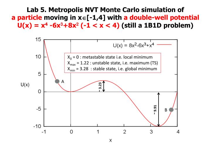
Lab 5. Metropolis NVT Monte Carlo simulation of a particle moving in x [-1,4] with a double-well potential U (x) = x 4 -6x 3 +8x 2 (-1 < x < 4) (still a 1B1D problem). X 0 = 0 : metastable state i.e. local minimum X max = 1.22 : unstable state, i.e. maximum (TS)

E N D
Lab 5. Metropolis NVT Monte Carlo simulation of a particle moving in x[-1,4] with a double-well potential U(x) = x4 -6x3+8x2 (-1 < x < 4) (still a 1B1D problem) X0 = 0 : metastable state i.e. local minimum Xmax = 1.22 : unstable state, i.e. maximum (TS) Xmin = 3.28 : stable state, i.e. global minimum A U(x) ~ 3.23 B ~ 9.91
How do we mimic the Mother Nature in a virtual space to realize lots of microstates, all of which correspond to a given macroscopic state? By MC or MD method! microscopic states (microstates) or microscopic configurations ~1023 particles t1 t2 t3 under external constraints (N or , V or P, T or E, etc.) Ensemble (micro-canonical, canonical, grand canonical, etc.) In a real-space experiment In a virtual-space simulation Average over a collection of microstates they’re generated naturally from thermal fluctuation it is us who needs to generate them by MC or MD methods. Macroscopic quantities (properties, observables) These are what are measured in true experiments. • thermodynamic – or N, E or T, P or V, Cv, Cp, H, S, G, etc. • structural – pair correlation function g(r), etc. • dynamical – diffusion, etc.
Beyond one-body problem. Two-body case first. Example of pairwise interaction potentials 1. • Based on Hooke's law (Simple harmonic functions). • Energy associated with vibration about the equilibrium bond length.
Bond Stretching Energy • Based on Hooke's law (Simple harmonic functions). • Energy associated with vibration about the equilibrium bond length. • "kb" parameter controls the stiffness of the bond spring (force constant). • "ro" parameter defines its equilibrium length. • "kb" & "ro" parameters are assigned to each pair of bonded atoms • based on their types (e.g. C-C, C-H, O-C, etc.). • The model breaks down as a bond is stretched toward the point of dissociation. • But bonds are usually so stiff that it works for moderate T.
Beyond one-body problem. Two-body case first. Example of pairwise interaction potentials 2. Pair-wise sum of the energies of all possible interacting non-bonded atoms i and j
Non-bonded Energy: van der Waals Attraction • Correlation of electron fluctuations. • Only attraction which is present between nonpolar molecules • (the reason that Ar, He, CH4 can form liquid phases) • Stronger for larger, more polarizable molecules. • e.g. CCl4 > CH4 ; Kr > Ar > He • a.k.a. “London” or “dispersion” forces Non-bonded Energy: van der Waals Repulsion • Overlap of electron clouds • Lennard-Jones Exp-6 (Buckingham)
Beyond one-body problem. Two-body case first. Example of pairwise interaction potentials 3. Non-bonded Energy: Electrostatic (Coulombic) Energy • Coulomb’s law • Variables: Interatomic distance (rij) • Parameters: atomic charges (qi) calculated using QM • Dielectric constant (0) for the attenuation of • electrostatic interaction by the environment • (80 for aq solution; 1 for vacuum) • Very long-range
Beyond two-body potential: Angle Bending Energy • Also based on Hooke's law (Harmonic function). • Energy associated with vibration about the equilibrium bond angle. • "kθ" parameter controls the stiffness of the angle spring (force constant). • "θo" parameter defines its equilibrium angle. • Parameters are assigned to each bonded triplet of atoms based on their types • (e.g. C-C-C, C-O-C, C-C-H, etc.).
Beyond two-body potential: Torsion (A-B-C-D bond) • Modeled by a simple periodic function • "A" parameter controls the amplitude of the curve. • "n" parameter controls its periodicity and reflects the symmetry in torsion angle. • "" parameter shifts the entire curve along the rotation angle axis (). • The parameters are determined from curve fitting. • Parameters are assigned to each bonded quartet of atoms based on their types • (e.g. C-C-C-C, C-O-C-N, H-C-C-H, etc.). • CH3-CH3, for example, ought to repeat its energy every 120. • The cis conformation of a dihedral angle is assumed to be the zero by convention.
Force Fields and Molecular Mechanics • Bypass the time-consuming QM procedure (ignore electrons) • Write E(R) as a parametric function of nuclear coordinates R • Derive the function E(R) from an intuitiveball-and-spring model • Fit the parameters to experiment and/or higher-level computational data
x E’ = ki (lil0,i) + ki’ (θi θ0,i) + etc… rij li bonds angles i E’’ = ki + ki’ + etc… θi bonds angles Potential energy surface, Force field & Molecular Mechanics • How do we obtain the potential energy E? • QM: Solve Schrödinger equation • MM: Evaluate analytic functions (FF) 3N (or 3N-6 or 3N-5) Dimension PES for N-atom system For geometry optimization, evaluate E, E’ (& E’’) at the input structure X (x1,y1,z1,…,xi,yi,zi,…,xN,yN,zN) or {li,θi,i}.
+ cross terms (coupling) Bonded interaction (valence terms) Nonbonded interaction (non-bonding term) van der Waals (dispersion) Coulombic interaction (electrostatic) Sum of individual components The mathematical form of the energy terms varies from force-field to force-field.
Bond Stretching Energy • Based on Hooke's law (Simple harmonic functions). • Energy associated with vibration about the equilibrium bond length. • "kb" parameter controls the stiffness of the bond spring (force constant). • "ro" parameter defines its equilibrium length. • "kb" & "ro" parameters are assigned to each pair of bonded atoms • based on their types (e.g. C-C, C-H, O-C, etc.). • The model breaks down as a bond is stretched toward the point of dissociation. • But bonds are usually so stiff that it works for moderate T.
Bond Stretching Energy • Taylor expansion of energy about equilibrium position ro higher term neglected minimum defined as 0 harmonic unrealistic when the bond is stretched. fails in strained geometries. Polynomial with higher terms The limiting behavior is not correct for 3rd, 5th order… Morse potential
Angle Bending Energy • Also based on Hooke's law (Harmonic function). • Energy associated with vibration about the equilibrium bond angle. • "kθ" parameter controls the stiffness of the angle spring (force constant). • "θo" parameter defines its equilibrium angle. • Parameters are assigned to each bonded triplet of atoms based on their types • (e.g. C-C-C, C-O-C, C-C-H, etc.).
q Angle Bending Energy • Taylor expansion of energy about equilibrium position • improvements by including higher-order terms • Out-of-plane bending higher term neglected minimum defined as 0 harmonic
Torsion Energy (for A-B-C-D bond) • Periodic • Weak (~100 times less stiff than bond stretching motions) • (Taylor expansion in f not appropriate) • Fourier series • Terms are included to capture appropriate minima/maxima • Depends on substituent atoms • e.g., ethane has three mimum-energy conformations (n = 3) • Depends on type of bond • e.g. ethane (CH3CH3) vs. ethylene (CH2CH2) • Usually at most n = 1, 2, and/or 3 terms are included
Torsion Energy (for A-B-C-D bond) • Modeled by a simple periodic function • "A" parameter controls the amplitude of the curve. • "n" parameter controls its periodicity and reflects the symmetry in torsion angle. • "" parameter shifts the entire curve along the rotation angle axis (). • The parameters are determined from curve fitting. • Parameters are assigned to each bonded quartet of atoms based on their types • (e.g. C-C-C-C, C-O-C-N, H-C-C-H, etc.). • CH3-CH3, for example, ought to repeat its energy every 120. • The cis conformation of a dihedral angle is assumed to be the zero by convention.
Non-bonded Energy Pair-wise sum of the energies of all possible interacting non-bonded atoms i and j
Non-bonded Energy: van der Waals Attraction • Correlation of electron fluctuations. • Only attraction which is present between nonpolar molecules • (the reason that Ar, He, CH4 can form liquid phases) • Stronger for larger, more polarizable molecules. • e.g. CCl4 > CH4 ; Kr > Ar > He • a.k.a. “London” or “dispersion” forces Non-bonded Energy: van der Waals Repulsion • Overlap of electron clouds • Lennard-Jones Exp-6 (Buckingham)
Non-bonded Energy: Electrostatic (Coulombic) Energy • Coulomb’s law • Variables: Interatomic distance (rij) • Parameters: atomic charges (qi) calculated using QM • Dielectric constant (0) for the attenuation of • electrostatic interaction by the environment • (80 for aq solution; 1 for vacuum) • Very long-range
5000-atom system x x x x Cutoff for Long-Range Non-bonded Interactions • Direct method (simplest) • Interactions are calculated to a cutoff distance. • Interactions beyond this distance are ignored. • Leads to discontinuities in energy and derivatives. • As a pair distance moves in and out of the cutoff • range between calculation steps, the energy jumps. • (since the non-bond energy for that pair is included • in one step and excluded from the next.)
Minimizing discontinuity. Spline, a possible choice Effective potential = actual potential smoothing function S(r) • Switching function S(r) • = 1 for small r • = 1 0 smoothly at intermediate r • = 0 for large r • Should be continuously differentiable • (so that forces can be calculated). • Smoothly turns off non-bond interactions over a range of distances. • Switching range is important. • Upper limit = the cut-off distance. • Too large lower limit (small spline width) Unrealistic forces may result. • Too small lower limit The feature of the equilibrium region may be lost.
Cutoff for Long-Range Non-bonded Interactions Number of non-bond interactions for a 5000-atom system as a function of cutoff distance vdW energy of a hexapeptide crystal as a function of cutoff distance, which does not converge until 20 Å
Estimating Non-bonded (esp. Electrostatic) Energy for Periodic Systems: Ewald Summation For details, read Leach (pp.324-343) and reading materials (Kofke)
Some Commonly Used Force Fields (Goddard) (Goddard) (Kollman)
Force Field Parametrization X-ray, neutron, electron diffraction, NMR (structure), Calorimetry (enegy), IR spectroscopy, elastic properties