Download
1 / 15
150 likes | 151 Vues
This chapter explains the general principles and different methods for cost estimation using regression equations, including engineering methods, inspection of accounts, graphical or scattergraph method, high-low method, and least squares method.

E N D
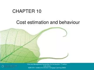
CHAPTER 10 Cost estimation and behaviour
10.1a General principles • A regression equation (or cost function) measures past relationships between a dependent variable (total cost)and potential independent variables (i.e. cost drivers/activity measures). • Simple regression y = a + bx Where y = Total cost a = Total fixed cost for the period b = Average unit variable cost x = Volume of activity or cost driver for the period • Multiple regression y = a + b1 x1 + b2 x2 • Resulting cost functions must make sense and be economicallyplausible.
10.1b • Cost estimation methods • Engineering methods • Inspection of accounts method • Graphical or scattergraph method • High-low method • Least squares method.
10.2 Engineering methods • Analysis based on direct observations of physical quantitiesrequired for an activity and then converted into costestimates. • Useful for estimating the costs of repetitive processes whereinput-output relationships are clearly defined. • Appropriate for estimating the costs associated with directlabour, materials and machine time. Inspection of accounts • Departmental manager and accountant inspect each itemof expenditure within the accounts for a particular periodand classify each item as fixed, variable or semi-variable.
10.3 Graphical or scattergraph method • Past observations are plotted on a graph and a line of best fit is drawn. • Unit VC = Difference in cost = £720 – £560 = £2 per hour Difference in activity 240 hours – 160 hours Figure 1 Graph of maintenance costs at different activity levels • Y = £240 + £2x
10.4a High–low method • Involves selecting the periods of highest and lowest activity levels and comparing changes in costs that result from the two levels. Example Lowest activity 5 000 units £22 000 Highest activity 10 000 units £32 000 Cost per unit = £10 000/5 000 units = £2 per unit Fixed costs = £22 000 – (5 000 × £2) = £12,000 • Major limitation = Reliance on two extreme observations
10.4b Figure 2 High–low method
10.5a The least squares regression formula Exhibit 1 Past observations of maintenance costs
10.5b The simple regression equation y = a + bx can be found from the following two equations and solving for a and b: The above equation can be used to predict costs at different output levels.
10.6a Multiple regression analysis
10.6b Multiple regression analysis (cont.)
10.7 • Factors to be considered when using • past data to estimate cost functions • Identify the potential activity bases (i.e. cost drivers) • The objective is to find the cost driver that has the greatest effect on cost. • • Ensure that the cost data and activity measures relate to the same period. • Some costs lag behind the associated activity measures (e.g. wages paid for the output of a previous period). • • Ensure that a sufficient number of observations are obtained. • • Ensure that accounting policies do not lead to distorted cost functions. • • Adjust for past changes so that all data relates to the circumstances of the planning horizon. • Adjust for inflation, technological changes and observations based on abnormal situations.
10.8 Summary 1. Select the dependent variable (y) to be predicted. 2. Select the potential cost drivers. 3. Plot the observations on a graph.* 4. Estimate the cost function. 5.Test the reliability of the cost function. Figure 3 Effect of extrapolation costs *Be aware of the dangers of predicting costs outside the relevant range.
10.9a • Tests of reliability • Tests of reliability indicate how reliable • potential cost drivers are in predicting the dependent variable. • The most simplistic approach is to plot the data for each potential cost driver and examine the distances from the straight line derived from the visual fit. • A more simplistic approach is to compute the coefficient of variation (known as r2). • See slide 9b for the calculation of r2 from the data shown on sheet 5a.
10.9b r so that r2 = (0.941)2 = 0.8861 r2 indicates that 88.61% of the variation in total cost is explained by the variation in the activity base and the remaining 11.39% by other factors. Therefore the higher the coefficient of variation the stronger the relationship between the dependent and independent variable.