Download
1 / 31
310 likes | 318 Vues
Independent Samples: Comparing Means. Lecture 37 Sections 11.1 – 11.2, 11.4 Tue, Nov 6, 2007. Independent Samples. In a paired study, two observations are made on each subject, producing one sample of bivariate data . Or we could think of it as two samples of paired data.

E N D
Independent Samples: Comparing Means Lecture 37 Sections 11.1 – 11.2, 11.4 Tue, Nov 6, 2007
Independent Samples • In a paired study, two observations are made on each subject, producing one sample of bivariate data. • Or we could think of it as two samples of paired data.
Independent Samples • Paired data are often “before” and “after” observations. • By comparing the mean before treatment to the mean after treatment, we can determine whether the treatment had an effect.
Independent Samples • On the other hand, with independent samples, there is no logical way to “pair” the data. • One sample might be from a population of males and the other from a population of females. • Or one might be the treatment group and the other the control group. • Furthermore, the samples could be of different sizes.
Independent Samples • We start with two populations. • Population 1 has mean 1 and st. dev. 1. • Population 2 has mean 2 and st. dev. 2. • We wish to compare 1 and 2. • We do so by taking samples and comparing sample meansx1 andx2.
Independent Samples • We will usex1 –x2 as an estimator of 1 – 2. • If we want to know whether 1 = 2, we test to see whether 1 – 2 = 0 by computingx1 –x2 and comparing it to 0.
The Distributions ofx1 andx2 • Let n1 and n2 be the sample sizes. • If the samples are large, thenx1 andx2 have (approx.) normal distributions. • However, if either sample is small, then we will need an additional assumption: • The population of the small sample(s) is normal. in order to use the t distribution.
Further Assumption • We will also assume that the two populations have the same standard deviation. • Call it . • That is, = 1 = 2. • If this assumption is not supported by the evidence, then it should not be made. • If this assumption is not made, then the formulas become much more complicated. See p. 658.
The Distribution ofx1 –x2 • If the sample sizes are large enough (or the populations are normal), then according to the Central Limit Theorem, • x1 has a normal distribution with mean 1and standard deviation 1/n1. • x2 has a normal distribution with mean 2 and standard deviation 2/n2.
The Distribution ofx1 –x2 • It follows from theory thatx1 –x2is • Normal, with • Mean • Variance
The Distribution ofx1 –x2 • If we assume that 1 = 2, (call it ), then the standard deviation may be simplified to • That is,
1 0 The Distribution ofx1
2 1 0 The Distribution ofx2
2 1 1– 2 0 The Distribution ofx1 –x2
The Distribution ofx1 –x2 • If then it follows that
Example • Work exercise 11.32 on page 716 under the assumption that = 6 for both populations.
The t Distribution • Let s1 and s2 be the sample standard deviations. • Whenever we use s1 and s2 instead of , then we will have to use the t distribution instead of the standard normal distribution, unless the sample sizes are large.
Estimating • Individually, s1 and s2 estimate . • However, we can get a better estimate than either one if we “pool” them together. • The pooled estimate is
x1 –x2 and the t Distribution • We should use t instead of Z if • We use sp instead of , and • The sample sizes are small. • The number of degrees of freedom is df = df1 + df2 = n1 + n2 – 2. • That is
Hypothesis Testing • See Example 11.4, p. 699 – Comparing Two Headache Treatments. • State the hypotheses. • H0: 1 = 2 • H1: 1 > 2 • State the level of significance. • = 0.05.
The t Statistic • Compute the value of the test statistic. • The test statistic is with df = n1 + n2 – 2.
Hypothesis Testing • Calculate the p-value. • The number of degrees of freedom is df = df1 + df2 = 18. • p-value = P(t > 1.416) = tcdf(1.416, E99, 18) = 0.0869.
Hypothesis Testing • State the decision. • Accept H0. • State the conclusion. • Treatment 1 is not more effective than Treatment 2.
The TI-83 and Means of Independent Samples • Enter the data from the first sample into L1. • Enter the data from the second sample into L2. • Press STAT > TESTS. • Choose either 2-SampZTest or 2-SampTTest. • Choose Data or Stats. • Provide the information that is called for. • 2-SampTTest will ask whether to use a pooled estimate of . Answer “yes.”
The TI-83 and Means of Independent Samples • Select Calculate and press ENTER. • The display shows, among other things, the value of the test statistic and the p-value.
Confidence Intervals • Confidence intervals for 1 – 2 use the same theory. • The point estimate isx1 –x2. • The standard deviation ofx1 –x2 is approximately
Confidence Intervals • The confidence interval is or or ( known, large samples) ( unknown, large samples) ( unknown, normal pops., small samples)
Confidence Intervals • The choice depends on • Whether is known. • Whether the populations are normal. • Whether the sample sizes are large.
Example • Find a 95% confidence interval for 1 – 2 in Example 11.4, p. 699. • x1 –x2 = 3.2. • sp = 5.052. • Use t = 2.101. • The confidence interval is 3.2 (2.101)(2.259) = 3.2 4.75.
The TI-83 and Means of Independent Samples • To find a confidence interval for the difference between means on the TI-83, • Press STAT > TESTS. • Choose either 2-SampZInt or 2-SampTInt. • Choose Data or Stats. • Provide the information that is called for. • 2-SampTTest will ask whether to use a pooled estimate of . Answer “yes.”