Download
1 / 35
470 likes | 848 Vues
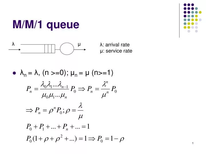
M/M/1 queue. λ n = λ , (n >=0); μ n = μ (n>=1). λ. μ. λ : arrival rate μ : service rate. Traffic intensity. rho = λ / μ It is a measure of the total arrival traffic to the system Also known as offered load Example: λ = 3/hour; 1/ μ =15 min = 0.25 h

E N D
M/M/1 queue • λn = λ, (n >=0); μn = μ (n>=1) λ μ λ: arrival rate μ: service rate
Traffic intensity • rho = λ/μ • It is a measure of the total arrival traffic to the system • Also known as offered load • Example: λ = 3/hour; 1/μ=15 min = 0.25 h • Represents the fraction of time a server is busy • In which case it is called the utilization factor • Example: rho = 0.75 = % busy
3 3 2 2 1 1 busy idle Queuing systems: stability N(t) • λ<μ • => stable system • λ>μ • Steady build up of customers => unstable 1 2 3 4 5 6 7 8 9 10 11 Time N(t) 1 2 3 4 5 6 7 8 9 10 11 Time
Example#1 • A communication channel operating at 9600 bps • Receives two type of packet streams from a gateway • Type A packets have a fixed length format of 48 bits • Type B packets have an exponentially distribution length • With a mean of 480 bits • If on the average there are • 20% type A packets and 80% type B packets • Calculate the utilization of this channel • Assuming the combined arrival rate is 15 packets/s
Performance measures • L • Mean # customers in the whole system • Lq • Mean queue length in the queue space • W • Mean waiting time in the system • Wq • Mean waiting time in the queue
Little’s theorem • This result • Existed as an empirical rule for many years • And was first proved in a formal way by Little in 1961 • The theorem • Relates the average number of customers L • In a steady state queuing system • To the product of the average arrival rate (λ) • And average waiting time (W) a customer spend in a system
LITTLE’s Formula • : average number of messages in system • : average delay • λ: arrival rate • Little’s relation holds for any • Service discipline • Arrival process • Holding area
Graphical Proof • A(t) • Cumulative arrival process • L(t) • Nb. of customers that left system up to t • => N(t) = A(t) – L(t) • Nb. of customers in system at time t • di: interval between ith arrival and its departure
Graphical Proof (continued) • Now, let
Mean waiting time (M/M/1) • Applying Little’s theorem
Z-transform: application in queuing systems • X is a discrete r.v. • P(X=i) = Pi, i=0, 1, … • P0 , P1 , P2 ,… • Properties of the z-transform • g(1) = 1, P0 = g(0); P1 = g’(0); P2 = ½ . g’’(0) • , +
M/M/1 Queue – Infinite Waiting Room • Probability generating function • Mean • Variance
M/M/S S servers μ λ
M/M/S: stable queue • is λ/Sμ < 1 ? • Otherwise you will not get a stable queue, as such
M/M/S: performance measures • Mean queue length • Mean waiting time in the queue (Little’s theorem) • Mean waiting time in the system • Mean # of customers in the whole system
Erlang C formula • A quantity of interest • Probability to find all s servers busy • Ratio between Lq and Pc
M/M/S: stability revisited • Stable • If λ/Sμ < 1 • Arrival rate to an individual server • Utilization of a server • Utilization of all servers
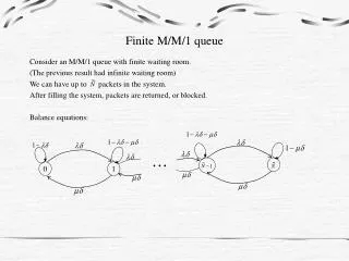
M/M/1/N • Birth and death equations λ μ % loss N
M/M/1/N: normalizing constant • Let ρ=λ/μ • As such Probability of arriving to a full waiting room
M/M/1/N: what percent of λ gets into the queue? • Percentage of time the queue is full • is equal to PN • Rate of lost customers = λ.PN • Rate of customers getting in : λ.(1-PN) • Often referred to as effectivecustomer arrival rate • Utilization of server .25 .75 Not full full
M/M/1/N: performance measures • Mean # of customers in the system • Mean queue length • Waiting time in system: W = L/λ • Waiting time in queue: Wq = Lq/λ LM/M./1
M/M/1/N: equivalent systems • When an M/M/1/N queue is full • Continuous arrival • A system with loss • is equivalent to shutting up the service • For the duration during which the queue is full • And starting it up again when system no longer ful • This system is called a shut down system • This equivalence holds only when • the inter-arrival is exponential
Proof: rate diagrams • M/M/1/N system with loss • Consider the special case where N = 5 λ λ λ λ λ λ 0 1 2 3 4 5 μ μ μ μ μ
Proof: rate diagrams (cont’d) • M/M/1/N shut down system • Consider the special case where N = 5 λ λ λ λ λ 0 1 2 3 4 5 μ μ μ μ μ
M/M/infinity: birth and death equations Infinite number of servers μ λ . .
Erlang system: M/M/S/S Finite number of Servers = S μ λ . .
Erlang loss formula Erlang loss formula • What percent gets in and • What percent gets lost • PS = prob S customers in system • Effective arrival rate • Rate of lost customers = λ.PS
Erlang B formula • Probability of finding all s servers busy • In an iterative form: