Download
1 / 42
430 likes | 668 Vues
9. Statistical Inference: Confidence Intervals and T-Tests. Suppose we wish to use a sample to estimate the mean of a population The sample mean will not necessarily be exactly the same as the population mean. Imagine that we take a sample of 3 from a population of 10,000 cases.

E N D
Suppose we wish to use a sample to estimate the mean of a population • The sample mean will not necessarily be exactly the same as the population mean. • Imagine that we take a sample of 3 from a population of 10,000 cases
Pop: 10,000 people with equal numbers of individuals with values of 1,2,3,4,5,6,7,8,9,10 S1: 1,2,9 mean=4 S2: 5,4,9 mean=6 S3: 3,7,5 mean=5 S4: 1,1,2 mean=1.3 S5: 7,9,5 mean=7 And so forth μ=5.5
Column one shows the population distribution Column two is the distribution of 3-draw means from column one; column three is the distribution of 30-draw means from column one. Distribution of Sample Mean by Same Size
Central Limit Theorem As Sample Size Gets Large Enough Sampling Distribution Becomes Almost Normal regardless of shape of population
Central Limit Theorem • For almost all populations, the sample mean is normally or approximately normally distributed, and the mean of this distribution is equal to the mean of the population and the standard deviation of this distribution can be obtained by dividing the population standard deviation by the square root of the sample size
If the original population is normal, a sample of only 1 case is normally distributed • The further the original sample is from normal, the larger the sample required to approach normality • Even for samples that are far from normal a modest number of cases will be approximately normal
When the Population is Normal Population Distribution Central Tendency _ = x Variation Sampling Distributions _ = x n = 4X = 5 n =16X = 2.5
When The Population is Not Normal Population Distribution Central Tendency = 10 Variation = 50 X Sampling Distributions n =30X = 1.8 n = 4X = 5
The Normal Distribution • Along the X axis you see Z scores, i.e. standardized deviations from the mean • Just think of Z scores as std. dev. denominated units. • A Z score tells us how many std. deviations a case lies above or below the mean
The Normal Distribution • Note a property of the Normal distribution • 68% of cases in a Normal distribution fall within 1 std. deviation of the mean • 95% within 2 std. dev. (actually 1.96) • 99.7% within 3 std. dev. • So what, you ask?
Welcome to Probability! • Probability is the likelihood of the occurrence of a single event • With just the mean and std. dev. of a (Normal) distribution we can make “inferences” using the Z score for any individual drawn randomly from the population. • E.g. Knowing that a salary survey of Americans reports a mean annual salary of 40,000 with a std. deviation of 10,000. What is the probability that a random person earns between 30K and 50K? • What’s the probability they earn over 50K?
Fun with standard normal probabilities! • Problem : • you are 78 inches (6’6”) tall & bet a friend that you are the tallest person on campus. Campus heights in inches are ~N (64, 10). What’s the probability that you’re wrong?
Confidence Intervals • We can use the Central Limit Theorem and the properties of the normal distribution to construct confidence intervals of the form: • The average salary is $40,000 plus or minus $1,000 with 95% confidence • Presidential support is 45% plus or minus 4% with 95% confidence. • In other words, we can make our best estimate using a sample and indicate a range of likely values for what we wish to estimate
Confidence Intervals • Notice that our estimates of the population parameter are probabilistic. • So we report our sample statistic with together with a measure of our (un)certainty • Most often, this takes the form of a 95 percent confidence interval establishing a boundary around the sample mean (x bar) which will contain the true population mean (μ) 95 out of 100 times.
Distribution of Confidence Intervals • S1 $40,000±$10,000 or $30,000 to $50,000 • S2 $36,000± $ 7,000 or $29,000 to $43,000 • S2 $42,000±$11,000 or $31,000 to $53,000 • S2 $41,000± $ 8,000 or $33,000 to $49,000 • Etc • 95% of the intervals we could draw will contain the true mean μ • If we draw one sample, as we almost always do the likelihood it will contain the true mean is .95
Now let’s look at how we can derive the confidence interval:
Confidence Intervals • Example: Randomly sampling 100 students for their GPA, you get a sample mean of 3.0 and a (pop) std. deviation of .4 • What is the 95% confidence interval? 1. Calculate the standard deviation for • Calculate the lower confidence boundary: 3.0 – (1.96*0.04) = 2.92 • Calculate the upper confidence boundary: 3.0 + (1.96*0.04) = 3.08 • You are 95% confident that the interval 3.0 +/- .08 or 2.92 to 3.08 contains the true student population mean GPA.
Standard Errors from Samples • Of course, life is usually not so simple. • As undeniably cool as the Central Limit Theorem is, however, it has a problem: • We need to know σ • How often do researchers really know the population std (σ) deviation needed for calculating standard errors? • Thank Guinness for the solution… Notation hint: population notation is mostly greek; sample latin.
How Guinness Saved the World • In the beginning of the 20th Century, a statistician at the Guinness Brewery in Dublin concerned with quality control came up with a solution • Calculate the standard deviation of the sample mean • and use Student’s t-distribution, which depends on sample size for inference. • Thank-you, Guinness! William Gosset, a.k.a. “Student”
The t-distribution • For samples under 120 or so, the difference between the sample distribution s and the normal distributionσcan be large, the smaller the sample the larger the difference • Solution: The t-distribution is flatter than the Z distribution and gets increasingly so as the sample shrinks. • Thus, the smaller the sample the larger the interval necessary for a given level of confidence. Small Sample? Hedge your bet!
t-table • No longer can we assume that the pop mean (μ) will be within 1.96 std. deviations of the sample mean in 95 out of 100 samples. • The smaller the sample the more std. deviations we can expect μ can be from x-bar at a given level of confidence. • Degrees of freedom capture the sample size, In our case= n - 1
Confidence Intervals w/out σ • Example: Randomly sampling 16 students for their GPA, you get a sample mean of 3.0 and sample std. deviation (s) of .4 • Identify an interval which will contain the true population mean 95% of the time. Calculate standard dev. of mean: • Calculate the interval 3 ±(2.145*.1)=3±.21 This is a confidence interval from 2.79 to 3.21. 95% of the time this interval will contain the mean. • If it were a known st. dev., σ, you would use the smaller value of z, 1.96 and the interval would be smaller: between 2.804 and 3.196.
Another exampleLet’s get back to our example! Sample of 15 students slept an average of 6.4 hours last night with standard deviation of 1 hour. Need t with n-1 = 15-1 = 14 d.f. For 95% confidence, t14 = 2.145
What happens to CI as sample gets larger? For large samples: Z and t values become almost identical, so CIs are almost identical.
Sample Proportions • What to do with dichotomous nominal variables. Often we wish to estimate a confidence interval for a proportion. For example 49% ± 4% approve of President Bush’s performance in office. (95% confidence interval) • For a proportion, the variance is determined by the value of the mean, which is the proportion expressed as a decimal. • p = # of respondents in a category / sample size (π unknown true value) • It is the same as a percentage expressed as a decimal—for the example above it would be .49 • St. Dev of π (true unknown proportion) is approx by sq root of p(1-p)/n • Use t if sample small and z if large
Conservative estimates of Proportions • If we wish to be conservative in estimating our confidence interval for proportions, we often use the maximum variance possible for proportions. That is .5*.5/n. • The square root of that is the standard deviation of p. • Using .5 maximizes p*(1-p)
Hypothesis tests • We can use the same logic to test hypotheses: Suppose we hypothesize that women are more likely to rate Pres. Clinton favorably on the thermometer scale than are men. A thermometer scale is an interval measure so it is appropriate to compare means.
Hyp: Mean women > men (Clinton ther score) • Null or Alternative hyp: Women ≤ men • Our hypothesis would say that if we take the mean for women on the thermometer score and subtract that for men, the difference should be positive. • It is also the case, that this distribution of mean differences is distributed normally with a true mean equal to the true but unknown mean difference between men and women. The exact nature of the variance is known as well. • We can use these characteristics to ask if the null is true how likely is it we would have observed the data in our sample. If the probability is low, then we can reject the null and accept our hypothesis. In other words the data will support our hypothesis.
Preclint mean scores • n mean s s/√n • Men 787 54.15 29.558 1.054 • Women 1007 56.52 29.772 .938 • T value deg free • -1.675 1694.325 • (Unequal variance assumed)
Now our sample size is large enough to use z • Let’s look in column 3 t=1.675 • P just under .05 • Why one-tail?
So then if the null were true: women≤men, the likelihood of drawing the sample of values in the 2004 NES was < .05. • Thus the null is quite unlikely given our data. With 95% confidence we can reject the null and accept our hypothesis: Women, on average, rated Clinton higher than did men.
Women Rate Clinton Differently than Men • Returning to our earlier example of the thermometer comparison between men and women. Suppose we had hypothesized: • Hyp: Mean women ≠ men (Clinton ther score) • Null or Alternative hyp: Women = men • If women equal men the mean difference between them would be 0. For a large sample size and a 95% confidence interval to reject the null we would need to be further than 1.96 standard deviations from the mean of 0.
t-Distribution Support Refute Refute -4 -3 -2 -1 0 1 2 3 4 observed t
SPSS will also show a probability value based on t. It assumes you want to do a two tail test like the one we just discussed Anytime our hypothesis specifies direction, eg, Meanw-Meanm>0 rather than simply Meanw-Meanm≠0 we can and should use a one tail test. For our one tail test example (Meanw-Meanm>0), we could reject the null if our sample was > than 1.645 standard deviations from the mean. In the two tail situation (Meanw-Meanm≠0) we cannot reject the null unless our sample is > than 1.96 standard deviations from the mean. When the one tail test is appropriate, using it (which we always should) makes it more likely we will reject the null and accept our hypothesis
Suppose our hypothesis that there is a difference between men and women is true, but that the difference was small. If we also had a small sample size, the variance of the sample mean could easily be large enough that we would be unlikely to reject the null. The difference would be too small to discern. We would not be able to say with any statistical significance that men were different from women in rating Clinton • Conversely, we might have a very large sample and be able to reject the null with confidence in most samples even if the true difference between men and women was real but too small to be a meaningful difference substantively.
Degree of Confidence • Using 95% confidence is the most common degree of confidence calculated • However, that is a rather arbitrary choice • If your sample is very large or s is very small so that s/√n is quite small, then you might want to use a 99% confidence interval z=2.58. • On the other hand, if your sample is small or s is large so that s/√n is very large then using a 95% degree of confidence might construct an interval so large it would not be very useful in indicating where the mean is likely to be. Here you might want to go to a 90% confidence interval with z=1.645