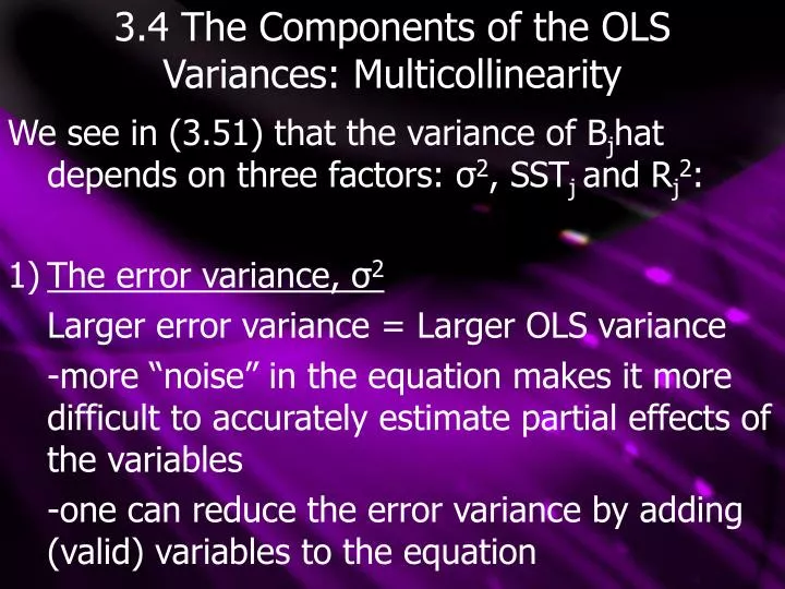
3.4 The Components of the OLS Variances: Multicollinearity

3.4 The Components of the OLS Variances: Multicollinearity We see in (3.51) that the variance of Bjhat depends on three factors: σ2, SSTj and Rj2: • The error variance, σ2 Larger error variance = Larger OLS variance -more “noise” in the equation makes it more difficult to accurately estimate partial effects of the variables -one can reduce the error variance by adding (valid) variables to the equation

3.4 The Components of the OLS Variances: Multicollinearity 2) The Total Sample Variation in xj, SSTj Larger xj variance – Smaller OLSj variance -increasing sample size keeps increasing SSTj since -This still assumes that we have a random sample

3.4 The Components of the OLS Variances: Multicollinearity 3) Linear relationships among x variables: Rj2 Larger correlation in x’s – Bigger OLSj variance -Rj2 is the most difficult component to understand - Rj2 differs from the typical R2 in that it measures the goodness of fit of: -Where xj itself is not considered an explanatory variable

3.4 The Components of the OLS Variances: Multicollinearity 3) Linear relationships among x variables: Rj2 -In general, Rj2 is the total variation in xj that is explained by the other independent variables -If Rj2=1, MLR.3 (and OLS) fails due to perfect multicollinearity (xj is a perfect linear combination of the other x’s) Note that: -High (but not perfect) correlation between independent variables is MULTICOLLINEARITY

3.4 Multicollinearity -Note that an Rj2 close to 1 DOES NOT violate MLR. 3 -unfortunately, the “problem” of multicollinearity is hard to define -No Rj2 is accepted as being too high -A high Rj2 can always be offset by a high SSTj or a low σ2 -Ultimately, how big is Bjhat relative to its standard error?

-Ceteris Paribus, it is best to have little correlation between xj and all other independent variables -Dropping independent variables will reduce multicollinearity -But if these variables are valid, we have created bias -Multicollinearity can always be fought by collecting more data -Sometimes multicollinearity is due to over specifying independent variables: 3.4 Multicollinearity

-In a study of heart disease, our economic model is: Heart disease=f(fast food, junk food, other) -Unfortunately, Rfast food2 is high, showing a high correlation between fast food and other x variables (especially junk food) -since fast food and junk food are so correlated, they should be examined together; their separate effects are difficult to calculate -Breaking up variables that can be added together can often cause Multicollinearity 3.4 Multicollinearity Example

3.4 Multicollineairity -it is important to note that multicollinearity may not affect ALL OLS estimates -take the following equation: -if x2 and x3 are correlated, Var(B2hat) and Var(B3hat) will be large (due to multicollinearity) -HOWEVER, from (3.51), if x1 is fully uncorrelated with x2 and x3, R12=0 and

3.4 Including Variables -Whether or not to include an independent variable is a balance between bias and variance: -take the following equation: -where both variables, x1 and x2, are included -Compare to the following equation with x2 omitted: If the true B2≠0 and x1 and x2 have ANY correlation, B1tilde is biased -Focusing on bias, B1hat is preferred

3.4 Including Variables -Considering variance complicates things -From (3.51), we know that: -Modifying a proof from chapter 2, we know that: -It is evident that unless x1 and x2 are uncorrelated in the sample, Var(B1tilde) is always smaller than Var(B1hat).

3.4 Including Variables -Obviously, if x1 and x2 aren’t correlated, we have no bias and no multicollinearity -If x1 and x2 are correlated: 1) If B2≠0, B1tilde is biased, B1hat is unbiased Var(B1tilde)< Var(B1hat) 2) If B2≠0, B1tilde is unbiased, B1hat is unbiased Var(B1tilde)< Var(B1hat) -Obviously in the second situation omit x2. If it has no real impact on y, adding it only causes multicollinearity and reduces OLS’s efficiency -Never include irrelevant variables

3.4 Including Variables -In the first case (B2≠0), leaving x2 out of the model results in a biased estimator of B1 -If the bias is small compared to the variance advantages, traditional econometricians have omitted x2 -However, 2 points argue for including x2: • Bias doesn’t shrink with n, but variance does • Error variance increases with omitted variables

3.4 Including Variables • Sample size, bias and variance -from discussion on (3.45), roughly bias doesn’t increase with sample size -from (3.51), increasing sample size increases SSTj and therefore decreases variance: -One can avoid bias and fight multicollinearity by increasing sample size

3.4 Including Variables 2) Error variance and omitted variables -When x2 is omitted and B2≠0, (3.55) underestimates error -Without including x2 in the model, x2’s variance is added to the error’s variance -higher error variance increases Bjhat’s variance

3.4 Estimating σ2 -In order to obtain unbiased estimators of Var(Bjhat), we must first find an unbiased estimator of σ2. -Since we know that σ2=E(u2), an unbiased estimator of σ2 would be: -Unfortunately, this is not a true estimator as we do not observe the errors ui.

3.4 Estimating σ2 -We know that errors and residuals can be written as: Therefore a natural estimate of σ2 would replace u with uhat -However, as seen in the bivariate case, this leads to bias, and we had to divide by n-2 to become a consistent estimator

3.4 Estimating σ2 -To make our estimate of σ2 consistent, we divide by the degrees of freedom n-k-1: Where k is the number of independent variables -Notice in the bivariate case k=1 and the denominator is n-2. Also note:

3.4 Estimating σ2 -Technically, n-k-1 comes from the fact that E(SSR=(n-k-1)σ2 -Intuitively, from OLS’s first order conditions: There are therefore k+1 restrictions on OLS residuals (j=1,2,…k) -If we therefore have n-(k+1) residuals we can use these restrictions to find the remaining residuals

Theorem 3.3(Unbiased Estimation of σ2) Under the Gauss-Markov Assumptions MLR. 1 through MLR. 5, Note: This proof requires matrix algebra and is found in Appendix E

Theorem 3.3 Notes -the positive square root of σhat2, σhat, is called the STANDARD ERROR OF THE REGRESSION (SER), or the STANDARD ERROR OF THE ESTIMATE -SER is an estimator of the standard deviation of the error term -when another independent variable is added to the equation, both SSR and the degrees of freedom fall -Therefore an additional variable may increase or decrease SER

Theorem 3.3 Notes In order to construct confidence intervals and perform hypothesis tests, we need the STANDARD DEVIATION OF BJHAT: Since σ is unknown, we replace it with its estimator, σhat, to give us the STANDARD ERROR OF BJHAT:

3.4 Standard Error Notes -since the standard error depends on σhat, it has a sampling distribution -Furthermore, standard error comes from the variance formula, which relies on homoskedasticity (MLR.5) -While heteroskedasticity doesn’t cause bias in Bjhat, it does affect its variance and therefore cause bias in its standard errors -Chapter 8 covers how to correct for heteroskedasticity

3.5 Efficiency of OLS - BLUE -MLR. 1 through MLR. 4 show that OLS is unbiased, but many unbiased estimators exist -HOWEVER, using MLR.1 through MLR.5, OLS’s estimate Bjhat of Bj is BLUE: Best Linear Unbiased Estimator

3.5 Efficiency of OLS - BLUE Estimator -OLS is an estimator as “it is a rule that can be applied to any sample of data to produce an estimate” Unbiased -Since OLS’s estimate has the property OLS is unbiased

3.5 Efficiency of OLS - BLUE Linear -OLS’s estimates are linear since Bjhat can be expressed as a linear function of the data on the dependent variable Where wij is a function of independent variables -This is evident from equation (3.22)

3.5 Efficiency of OLS - BLUE Best -OLS is best since it has the smallest variance of all linear unbiased estimators The Gauss-Markov theorem states that, given assumptions MLR. 1 through MLR.5, for any other estimator Bjtilde that is linear and unbiased: And this equality is generally strict

Theorem 3.4(Gauss-Markov Theorem) Under the Assumptions MLR. 1 through MLR. 5, Are respectively the best linear unbiased estimators (BLUE’s) of

Theorem 3.4 Notes -if our assumptions hold, no linear unbiased estimator will be a better choice than OLS -if we find any other unbiased linear estimator, its variance will be at least as big as OLS’s -If MLR.4 fails, OLS is biased and Theorem 3.4 fails -If MLR.5 (homoskedasticity) fails, OLS is not biased but no longer has the smallest variance, it is LUE

3.4 The Components of the OLS Variances: Multicollinearity