Download
1 / 44
440 likes | 702 Vues
Index construction. 4 장. Plan. Tolerant retrieval Wildcards Spell correction Soundex This time: Index construction. Index construction. How do we construct an index? What strategies can we use with limited main memory?. Our corpus for this lecture. Reuters-RCV1 collection

E N D
Plan • Tolerant retrieval • Wildcards • Spell correction • Soundex • This time: • Index construction
Index construction • How do we construct an index? • What strategies can we use with limited main memory?
Our corpus for this lecture • Reuters-RCV1 collection • Number of docs = n = 1M • Each doc has 1K terms • Number of distinct terms = m = 500K • 667 million postings entries
How many postings? • Number of 1’s in the i th block = nJ/i • Summing this over m/J blocks, we have • For our numbers, this should be about 667 million postings.
Recall index construction • Documents are parsed to extract words and these are saved with the Document ID. Doc 1 Doc 2 I did enact Julius Caesar I was killed i' the Capitol; Brutus killed me. So let it be with Caesar. The noble Brutus hath told you Caesar was ambitious
After all documents have been parsed the inverted file is sorted by terms. Key step We focus on this sort step. We have 667M items to sort.
Index construction • As we build up the index, cannot exploit compression tricks • Parse docs one at a time. • Final postings for any term – incomplete until the end. • (actually you can exploit compression, but this becomes a lot more complex) • At 10-12 bytes per postings entry, demands several temporary gigabytes
System parameters for design • Disk seek ~ 10 milliseconds • Block transfer from disk ~ 1 microsecond per byte (following a seek) • All other ops ~ 10 microseconds • E.g., compare two postings entries and decide their merge order
Bottleneck • Parse and build postings entries one doc at a time • Now sort postings entries by term (then by doc within each term) • Doing this with random disk seeks would be too slow – must sort N=667M records If every comparison took 2 disk seeks, and N items could be sorted with N log2N comparisons, how long would this take?
Sorting with fewer disk seeks • 12-byte (4+4+4) records (term, doc, freq). • These are generated as we parse docs. • Must now sort 667M such 12-byte records by term. • Define a Block ~ 10M such records • can “easily” fit a couple into memory. • Will have 64 such blocks to start with. • Will sort within blocks first, then merge the blocks into one long sorted order.
Sorting 64 blocks of 10M records • First, read each block and sort within: • Quicksort takes 2N ln N expected steps • In our case 2 x (10M ln 10M) steps • Exercise: estimate total time to read each block from disk and and quicksort it. • 64 times this estimate - gives us 64 sorted runs of 10M records each. • Need 2 copies of data on disk, throughout.
1 3 2 4 Merging 64 sorted runs • Merge tree of log264= 6 layers. • During each layer, read into memory runs in blocks of 10M, merge, write back. 2 1 Merged run. 3 4 Runs being merged. Disk
Merge tree 1 run … ? 2 runs … ? 4 runs … ? 8 runs, 80M/run 16 runs, 40M/run … 32 runs, 20M/run Bottom level of tree. Sorted runs. … 1 2 63 64
Merging 64 runs • Time estimate for disk transfer: • 6 x (64runs x 120MB x 10-6sec) x 2 ~ 25hrs. Disk block transfer time.Why is this an Overestimate? Work out how these transfers are staged, and the total time for merging. # Layers in merge tree Read + Write
Blocked sort-based indexing • Merge 방법을 잘 쓰면 효과적이지만, 역시 추가 2 path이므로 속도가 느림 • 현재 미리내시스템의 구현 방법임 • 내부정렬 방법은 fast-quick sorting • 외부정렬은 m-way merge sorting • Merge 이전에 모든 term을 앎
Exercise - fill in this table Step Time 1 64 initial quicksorts of 10M records each Read 2 sorted blocks for merging, write back 2 3 Merge 2 sorted blocks ? 4 Add (2) + (3) = time to read/merge/write 5 64 times (4) = total merge time
Single-path in memory indexing • 그림4.4 • 빈 사전에서 출발하여 사전에 term을 추가하면서 진행 • 따라서 순서가 처음 term이 보인 순서로 사전에 저장 • Posting을 새로 만들 때는 조금의 memory를 배정하고, 꽉 차면 2배로 키워 감 • 사전에 posting의 길이를 모름 • Term이 나타나면 사전에 있는지를 보고 없으면 사전에 추가, 있으면 posting만 추가 • 마지막에 사전을 알파벳 순서로 정렬
장단점 분석 • 한 번만 보고, 정렬 없이(사전은 제외) 처리하므로 속도가 빠름 • 주기억장치의 메모리가 작아도 괜찮음 • 작다고 해도 일반적으로 Giga-bytes 이상 (일반적인 IR) • O(T) • 압축을 한다면… • 압축에 대한 차이 설명
Large memory indexing • Suppose instead that we had 16GB of memory for the above indexing task. • Exercise: What initial block sizes would we choose? What index time does this yield? • Repeat with a couple of values of n, m. • In practice, spidering often interlaced with indexing. • Spidering bottlenecked by WAN speed and many other factors - more on this later.
Distributed indexing • For web-scale indexing (don’t try this at home!): must use a distributed computing cluster • Individual machines are fault-prone • Can unpredictably slow down or fail • How do we exploit such a pool of machines?
Distributed indexing • Maintain a master machine directing the indexing job – considered “safe”. • Break up indexing into sets of (parallel) tasks. • Master machine assigns each task to an idle machine from a pool.
Parallel tasks • We will use two sets of parallel tasks • Parsers • Inverters • Break the input document corpus into splits • Each split is a subset of documents • Master assigns a split to an idle parser machine • Parser reads a document at a time and emits (term, doc) pairs
Parallel tasks • Parser writes pairs into j partitions • Each for a range of terms’ first letters • (e.g., a-f, g-p, q-z) – here j=3. • Now to complete the index inversion
Data flow Master assign assign Postings Parser Inverter a-f g-p q-z a-f Parser a-f g-p q-z Inverter g-p Inverter splits q-z Parser a-f g-p q-z
Inverters • Collect all (term, doc) pairs for a partition • Sorts and writes to postings list • Each partition contains a set of postings Above process flow a special case of MapReduce.
Dynamic indexing • Docs come in over time • postings updates for terms already in dictionary • new terms added to dictionary • Docs get deleted
Simplest approach • Maintain “big” main index • New docs go into “small” auxiliary index • Search across both, merge results • Deletions • Invalidation bit-vector for deleted docs • Filter docs output on a search result by this invalidation bit-vector • Periodically, re-index into one main index
다른 방법 • 주기억장치의 posting의 크기가 일정 크기를 넘으면 하드디스크에 추가 • O(T2/n) • 옮길 때 단계를 둠 • O(T*log(T/n))
Issue with big and small indexes • Corpus-wide statistics are hard to maintain • E.g., when we spoke of spell-correction: which of several corrected alternatives do we present to the user? • We said, pick the one with the most hits • How do we maintain the top ones with multiple indexes? • One possibility: ignore the small index for such ordering • Will see more such statistics used in results ranking
Building positional indexes • Still a sorting problem (but larger) • Exercise: given 1GB of memory, how would you adapt the block merge described earlier? Why?
추가 • docID가 아니라 빈도순 • Security
Building n-gram indexes • As text is parsed, enumerate n-grams. • For each n-gram, need pointers to all dictionary terms containing it – the “postings”. • Note that the same “postings entry” can arise repeatedly in parsing the docs – need efficient “hash” to keep track of this. • E.g., that the trigram uou occurs in the term deciduous will be discovered on each text occurrence of deciduous
Building n-gram indexes • Once all (n-gramterm) pairs have been enumerated, must sort for inversion • Recall average English dictionary term is ~8 characters • So about 6 trigrams per term on average • For a vocabulary of 500K terms, this is about 3 million pointers – can compress
Index on disk vs. memory • Most retrieval systems keep the dictionary in memory and the postings on disk • Web search engines frequently keep both in memory • massive memory requirement • feasible for large web service installations • less so for commercial usage where query loads are lighter
Indexing in the real world • Typically, don’t have all documents sitting on a local filesystem • Documents need to be spidered • Could be dispersed over a WAN with varying connectivity • Must schedule distributed spiders • Have already discussed distributed indexers • Could be (secure content) in • Databases • Content management applications • Email applications
Content residing in applications • Mail systems/groupware, content management contain the most “valuable” documents • http often not the most efficient way of fetching these documents - native API fetching • Specialized, repository-specific connectors • These connectors also facilitate document viewing when a search result is selected for viewing
Secure documents • Each document is accessible to a subset of users • Usually implemented through some form of Access Control Lists (ACLs) • Search users are authenticated • Query should retrieve a document only if user can access it • So if there are docs matching your search but you’re not privy to them, “Sorry no results found” • E.g., as a lowly employee in the company, I get “No results” for the query “salary roster”
Users in groups, docs from groups • Index the ACLs and filter results by them • Often, user membership in an ACL group verified at query time – slowdown Documents Users 0/1 0 if user can’t read doc, 1 otherwise.
Exercise • Can spelling suggestion compromise such document-level security? • Consider the case when there are documents matching my query, but I lack access to them.
Compound documents • What if a doc consisted of components • Each component has its own ACL. • Your search should get a doc only if your query meets one of its components that you have access to. • More generally: doc assembled from computations on components • e.g., in Lotus databases or in content management systems • How do you index such docs? No good answers …
“Rich” documents • (How) Do we index images? • Researchers have devised Query Based on Image Content (QBIC) systems • “show me a picture similar to this orange circle” • watch for lecture on vector space retrieval • In practice, image search usually based on meta-data such as file name e.g., monalisa.jpg • New approaches exploit social tagging • E.g., flickr.com
Passage/sentence retrieval • Suppose we want to retrieve not an entire document matching a query, but only a passage/sentence - say, in a very long document • Can index passages/sentences as mini-documents – what should the index units be? • This is the subject of XML search
Resources • MG Chapter 5