Download
1 / 45
460 likes | 568 Vues
Index Construction. Recap. Inverted index. Recap. parsing Problems in “equivalence classing” A term is an equivalence class of tokens. How do we define equivalence classes? Case folding Stemming, Porter stemmer Posting list usage

E N D
Index Construction L06IndexConstruction
Recap • Inverted index
Recap • parsing • Problems in “equivalence classing” • A term is an equivalence class of tokens. • How do we define equivalence classes? • Case folding • Stemming, Porter stemmer • Posting list usage • How can we make intersecting postings lists more efficient • Skip pointers • How to support Phrase query • K-gram • Biword indexes • Positional indexes
Recap • Dictionary • Dictionary as array of fixed-width entries • Look up • Hash • B+-tree • Wildcard queries • Permuterm index • K-gram • spelling correction • Edit distance • Jaccard coefficient
Hardware basics • Many design decisions in information retrieval are based on hardware constraints. • We begin by reviewing hardware basics that we’ll need in this course.
Hardware basics • Access to data is much faster in memory than on disk. (roughly a factor of 10) • Disk seeks: No data is transferred from disk while the disk head is being positioned. • Therefore: Transferring one large chunk of data from disk to memory is faster than transferring many small chunks. • Disk I/O is block-based: Reading and writing of entire blocks (as opposed to smaller chunks). • Block sizes: 8KB to 256 KB • Servers used in IR systems typically have several GB of main memory, sometimes tens of GB. Available disk space is several orders of magnitude larger.
Index construction • How do we construct an index? • What strategies can we use with limited main memory? • How can we construct an index for very large collections? • Taking into account the hardware constraints • Memory, disk, speed etc.
Recall index construction • Documents are parsed to extract words and these are saved with the Document ID. Doc 1 Doc 2 I did enact Julius Caesar I was killed i' the Capitol; Brutus killed me. So let it be with Caesar. The noble Brutus hath told you Caesar was ambitious
After all documents have been parsed the inverted file is sorted by terms. Key step We focus on this sort step. We have lots of items to sort.
Sort-based index construction • As we build index, we parse docs one at a time. • The final postings for any term are incomplete until the end. • At 10–12 bytes per postings entry, demands a lot of space for large collections. • T = 100,000,000 in the case of RCV1 • Actually, we can do 100,000,000 in memory, but typical collections are much larger than RCV1. • Thus: We need to store intermediate results on disk.
Same algorithm for disk? • Can we use the same index construction algorithm for larger collections, but by using disk instead of memory? • No! • Sorting T = 100,000,000 records on disk is too slow – too many disk seeks. • We need an external sorting algorithm.
“External” sorting algorithm (using few disk seeks) • 12-byte (4+4+4) postings (termID, docID, document frequency) • Term -> termID (for efficiency) • Must now sort T = 100,000,000 such 12-byte postings by termID • Define a block to consist of 10,000,000 such postings • We can easily fit that many postings into memory. • We will have 10 such blocks for RCV1. • Basic idea of algorithm: • Accumulate postings for each block, sort, write to disk. • Then merge the blocks into one long sorted order.
2-Way Sort: Requires 3 Buffers • Pass 1: Read a page, sort it, write it. • only one buffer page is used • Pass 2, 3, …, etc.: • three buffer pages used. INPUT 1 OUTPUT INPUT 2 Main memory buffers Disk Disk
Two-Way External Merge Sort 6,2 2 Input file 3,4 9,4 8,7 5,6 3,1 • Each pass we read + write each page in file. • N pages in the file => the number of passes • So toal cost is: • Idea:Divide and conquer: sort subfiles and merge PASS 0 1,3 2 1-page runs 3,4 2,6 4,9 7,8 5,6 PASS 1 4,7 1,3 2,3 2-page runs 8,9 5,6 2 4,6 PASS 2 2,3 4,4 1,2 4-page runs 6,7 3,5 6 8,9 PASS 3 1,2 2,3 3,4 8-page runs 4,5 6,6 7,8 9
General External Merge Sort • More than 3 buffer pages. How can we utilize them? • To sort a file with N pages using B buffer pages: • Pass 0: use B buffer pages. Produce sorted runs of B pages each. • Pass 2, …, etc.: merge B-1 runs. INPUT 1 . . . . . . INPUT 2 . . . OUTPUT INPUT B-1 Disk Disk B Main memory buffers
Cost of External Merge Sort • Number of passes: • Cost = 2N * (# of passes) • E.g., with 5 buffer pages, to sort 108 page file: • Pass 0: = 22 sorted runs of 5 pages each (last run is only 3 pages) • Pass 1: = 6 sorted runs of 20 pages each (last run is only 8 pages) • Pass 2: 2 sorted runs, 80 pages and 28 pages • Pass 3: Sorted file of 108 pages
Problem with sort-based algorithm • Our assumption was: we can keep the dictionary in memory. • We need the dictionary (which grows dynamically) in order to implement a term to termID mapping. • Actually, we could work with term,docID postings instead of termID,docID postings . . . • . . . but then intermediate files become very large. (We would end up with a scalable, but very slow index construction method.)
Single-pass in-memory indexing • Abbreviation: SPIMI • Key idea 1: Generate separate dictionaries for each block – no need to maintain term-termID mapping across blocks. • Key idea 2: Accumulate postings in postings lists as they occur. • With these two ideas we can generate a complete inverted index for each block. • These separate indexes can then be merged into one big index.
SPIMI: Compression • Compression makes SPIMI even more efficient. • Compression of terms • Compression of postings • Discuss in next lecture
Distributed indexing • For web-scale indexing, must use a distributed computer cluster • Individual machines are fault-prone. • Can unpredictably slow down or fail. • How do we exploit such a pool of machines?
Google data centers • Google data centers mainly contain commodity machines. • Data centers are distributed all over the world. • Estimate: a total of 1 million servers, 3 million processors • Estimate: Google installs 100,000 servers each quarter. • Based on expenditures of 200–250 million dollars per year • What is the expected number of servers failing per minute for an installation of 1 million servers?
Distributed indexing • Maintain a master machine directing the indexing job –considered “safe” • Break up indexing into sets of parallel tasks • Master machine assigns each task to an idle machine from a pool.
Parallel tasks • We will define two sets of parallel tasks and deploy two types of machines to solve them: • Parsers • Inverters • Break the input document collection into splits (corresponding to blocks in BSBI/SPIMI) • Each split is a subset of documents.
Parsers • Master assigns a split to an idle parser machine. • Parser reads a document at a time and emits (term,doc) pairs. • Parser writes pairs into j term-partitions. • Each for a range of terms’ first letters • E.g., a-f, g-p, q-z (here: j = 3)
Inverters • An inverter collects all (term,doc) pairs (= postings) for one term-partition. • Sorts and writes to postings lists • Each partition contains a set of postings
Data flow Master assign assign Postings Parser Inverter a-f g-p q-z a-f Parser a-f g-p q-z Inverter g-p Inverter splits q-z Parser a-f g-p q-z
Dynamic indexing • Up to now, we have assumed that collections are static. • They rarely are. • Documents are inserted, deleted and modified. • postings updates or deletes for terms already in dictionary • new terms added to dictionary • This means that the dictionary and postings lists have to be modified
Simplest approach • Maintain “big” main index on disk • New docs go into “small” auxiliary index in memory. • Search across both, merge results • Periodically, merge auxiliary index into one main index • Deletions: • Invalidation bit-vector for deleted docs • Filter docs returned by index using this invalidation bit-vector; only return “valid” docs to user
Issue with auxiliary and main index • Frequent merges • Poor performance during merge • Actually: • Merging of the auxiliary index into the main index is efficient if we keep a separate file for each postings list. • But then we would need a lot of files – inefficient.
Logarithmic merge • Maintain a series of indexes, each twice as large as the previous one. • Keep smallest (Z0) in memory • Larger ones (I0, I1, . . . ) on disk • If Z0 gets too big (> n), write to disk as I0 • or merge with I0 (if I0 already exists) and write merger to I1 etc.
Dynamic indexing at large search engines • Often a combination • Frequent incremental changes • Occasional complete rebuild
Building positional indexes • Basically the same problem except that the intermediate data structures are large.
“Rich” documents • (How) Do we index images? • Researchers have devised Query Based on Image Content (QBIC) systems • “show me a picture similar to this orange circle” • (see, vector space retrieval) • In practice, image search usually based on meta-data such as file name e.g., monalisa.jpg