Download

1 / 61
680 likes | 1.46k Vues
All Pair Shortest Path. IOI/ACM ICPC Training June 2004. All Pair Shortest Path. Note: Dijkstra ’ s Algorithm takes O((V+E)logV) time All Pair Shortest Path Problem can be solved by executing Dijkstra ’ s Algorithm |V| times Running Time: O(V(V+E)log V) Floyd-Warshall Algorithm: O(V 3 ).

E N D
All Pair Shortest Path IOI/ACM ICPC Training June 2004
All Pair Shortest Path • Note: Dijkstra’s Algorithm takes O((V+E)logV) time • All Pair Shortest Path Problem can be solved by executing Dijkstra’s Algorithm |V| times • Running Time: O(V(V+E)log V) • Floyd-Warshall Algorithm: O(V3)
Idea • Label the vertices with integers 1..n • Restrict the shortest paths from i to j to consist of vertices 1..k only (except i and j) • Iteratively relax k from 1 to n. k j i
Definition • Find shortest distance from i to j using vertices 1 .. k only k j i
Example 2 4 2 4 1 1 1 3 3 5 1 3 5 1
i = 4, j = 5, k = 0 2 4 2 4 1 1 1 3 3 5 1 3 5 1
i = 4, j = 5, k = 1 2 4 2 4 1 1 1 3 3 5 1 3 5 1
i = 4, j = 5, k = 2 2 4 2 4 1 1 1 3 3 5 1 3 5 1
i = 4, j = 5, k = 3 2 4 2 4 1 1 1 1 3 5 1 3 5 1
Idea k j i
The tables i k i j j k k=4 k=5
The code for i = 1 to |V| for j = 1 to |V| a[i][j][0] = cost(i,j) for k = 1 to |V| for i = 1 to |V| for j = 1 to |V| a[i][j][k] = min( a[i][j][k-1], a[i][k][k-1] + a[k][j][k-1])
Topological sort IOI/ACM ICPC Training June 2004
b d a c e Topological order • Consider the prerequisite structure for courses: • Each node x represents a course x • (x, y) represents that course x is a prerequisite to course y • Note that this graph should be a directed graph without cycles. • A linear order to take all 5 courses while satisfying all prerequisites is called a topological order. • E.g. • a, c, b, e, d • c, a, b, e, d
Topological sort • Arranging all nodes in the graph in a topological order • Applications: • Schedule tasks associated with a project
Topological sort algorithm Algorithm topSort1 n = |V|; Let R[0..n-1] be the result array; for i = 1 to n { select a node v that has no successor; R[n-i] = v; delete node v and its edges from the graph; } return R;
b a c e • d has no successor! Choose d! • Both b and e have no successor! Choose e! b b d b a a a a c c e • Both b and c have no successor! Choose c! • Only b has no successor! Choose b! • Choose a! • The topological order is a,b,c,e,d Example
Time analysis • Finding a node with no successor takes O(|V|+|E|) time. • We need to repeat this process |V| times. • Total time = O(|V|2 + |V| |E|). • We can implement the above process using DFS. The time can be improved to O(|V| + |E|).
Algorithm based on DFS Algorithm topSort2 s.createStack(); for (all nodes v in the graph) { if (v has no predecessors) { s.push(v); mark v as visited; } } while (s is not empty) { let v be the node on the top of the stack s; if (no unvisited nodes are children to v) {// i.e. v has no unvisited successor aList.add(1, v); s.pop();// blacktrack } else { select an unvisited child u of v; s.push(u); mark u as visited; } } return aList;
Bipartite Matching IOI/ACM ICPC Training June 2004
Definitions Matching Free Vertex
Definitions • Maximum Matching: matching with the largest number of edges
Definition • Note that maximum matching is not unique.
Intuition • Let the top set of vertices be men • Let the bottom set of vertices be women • Suppose each edge represents a pair of man and woman who like each other • Maximum matching tries to maximize the number of couples!
Applications • Matching has many applications. For examples, • Comparing Evolutionary Trees • Finding RNA structure • … • This lecture lets you know how to find maximum matching.
Alternating Path • Alternating between matching and non-matching edges. a c d e b f h i j g d-h-e: alternating path a-f-b-h-d-i: alternating path starts and ends with free vertices f-b-h-e: not alternating path e-j: alternating path starts and ends with free vertices
Idea • “Flip” augmenting path to get better matching • Note: After flipping, the number of matched edges will increase by 1!
Idea • Theorem (Berge 1975): A matching M in G is maximum iffThere is no augmenting path Proof: • () If there is an augmenting path, clearly not maximum. (Flip matching and non-matching edges in that path to get a “better” matching!)
Proof for the other direction • () Suppose M is not maximum. Let M’ be a maximum matching such that |M’|>|M|. • Consider H = MM’ = (MM’)-(MM’)i.e. a set of edges in M or M’ but not both • H has two properties: • Within H, number of edges belong to M’ > number of edges belong to M. • H can be decomposed into a set of paths. All paths should be alternating between edges in M and M’. • There should exist a path with more edges from M’. Also, it is alternating.
Idea of Algorithm • Start with an arbitrary matching • While we still can find an augmenting path • Find the augmenting path P • Flip the edges in P
Labelling Algorithm • Start with arbitrary matching
Labelling Algorithm • Pick a free vertex in the bottom
Labelling Algorithm • Run BFS
Labelling Algorithm • Alternate unmatched/matched edges
Labelling Algorithm • Until a augmenting path is found
Repeat • Pick another free vertex in the bottom
Repeat • Run BFS
Repeat • Flip
Answer • Since we cannot find any augmenting path, stop!
Overall algorithm • Start with an arbitrary matching (e.g., empty matching) • Repeat forever • For all free vertices in the bottom, • do bfs to find augmenting paths • If found, then flip the edges • If fail to find, stop and report the maximum matching.
Time analysis • We can find at most |V| augmenting paths (why?) • To find an augmenting path, we use bfs! Time required = O( |V| + |E| ) • Total time: O(|V|2 + |V| |E|)
Improvement • We can try to find augmenting paths in parallel for all free nodes in every iteration. • Using such approach, the time complexity is improved to O(|V|0.5 |E|)
Weighted Bipartite Graph 3 4 6 6
Weighted Matching Score: 6+3+1=10 3 4 6 6
Maximum Weighted Matching Score: 6+1+1+1+4=13 3 4 6 6
Augmenting Path (change of definition) • Any alternating path such that total score of unmatched edges > that of matched edges • The score of the augmenting path is • Score of unmatched edges – that of matched edges 3 4 6 6 Note: augmenting path need not start and end at free vertices!
Idea for finding maximum weight matching • Theorem: Let M be a matching of maximum weight among matchings of size |M|. • If P is an augmenting path for M of maximum weight, • Then, the matching formed by augmenting M by P is a matching of maximum weight among matchings of size |M|+1.