Download
1 / 17
190 likes | 507 Vues
Universal Soil Loss Equation. Environmental Applications of GIS 3-3-2009. Soil Erosion in GIS. Universal Soil Loss Equation (USLE), an empirical equation designed for the computation of average soil loss in agricultural fields. A = R*K*L*S*C*P

E N D
Universal Soil Loss Equation Environmental Applications of GIS 3-3-2009
Soil Erosion in GIS • Universal Soil Loss Equation (USLE), an empirical equation designed for the computation of average soil loss in agricultural fields. • A = R*K*L*S*C*P • A: potential long term average annual soil loss in tons per acre per year. (Ton/acre-yr) • R = rainfall and runoff factor, the greater the intensity and duration of the rain storm, the higher the erosion potential • K = soil erodibility factor (from Statesgo soil layer) • LS = slope length-gradient factor. Represents a ratio of soil loss under given conditions to that at a site with the “standard” slope steepness of 9% and slope length of 72.6 ft. The steeper and longer the slope, the higher the risk for erosion.
Soil Survey Geographic (SSURGO) Database • Access via Soil Data Mart (http://soildatamart.nrcs.usda.gov) • Select State | County | Download Data • “Submit Request” • Enter email address • Wait for the Notice.
USLE - factors • C: crop/vegetation management factor. It is used to determine the relative effectiveness of soil and crop management systems in terms of preventing soil loss. • For example: Corn : 0.40, Fruit Tree: 0.1, Hay and Pasture: 0.02 (see slide 13) • P: Support practice factor. It reflects the effects of practices that will reduce the amount and rate of water runoff and thus reduce the amount of erosion. Most common used supporting cropland practices are cross slope cultivation, contour farming and strip cropping. • Up & Down Slope: 1.0, Cross Slope: 0.75, Contour Farming: 0.50, Strip Cropping: 0.37, Strip cropping and contour: 0.25.
Soil Loss Tolerance Rates • A tolerable soil loss is the maximum annual amount of soil, which can be removed before the long term soil productivity is adversely affected. TN is 5 tons/acre/year • Generally, soils with deep, uniform, stone free topsoil materials and/or not previous eroded have been assumed to have a higher rate
Rainfall Erosivity Factor, R • Erosivity of rainfall events and is defined as the product of two rainstorm characteristics: kinetic energy and the maximum 30 minute intensity. (Kirkby and Morgan, 1980) • E = 1.213 + 0.89 logI • Where E = the kinetic energy, kg-m/m2 mm, • I = rainfall intensity, mm/hr • I30 = the maximum 30-minute rainfall intensity for the storm, mm/hr • Tj = the time period of the specific storm increment, hr. • And, jis the specific storm increment, n is the number of storm increments in a year.
Rainfall Data • http://www.ncdc.noaa.gov/oa/ncdc.html • Click “Free Data” | “Free Data B” | “Individual Station”, You may enter COOP ID for Monterey (406170) and select 15 minute precipitation data. • Enter email address and wait for the response for downloading the data. • Download textfile and save it as “monterey.txt” • Use Excel to open the file (may come with comma delimited)
Processing Data • Keep MO/DA/TIME/VALUE. • Check Values in at TIME=2500, If TIME=2500, then delete rows associated with that date. • How many days with precipitation > 0? • Total amount of precipitation in 2008? (unit: 1/100 inches) • In mm? • (This is a simplified data), the actual total rainfall is 31.8 inches from this station, Max. I30 is 0.8 inches (extrapolation factor: 1.88)
Rainfall Erosivity, R • You should get 2180 for E (partial value), multiplied by 1.88 (factor), then by 20.3 (0.8*25.4) I30 in mm, then divided by 173.6. • So, we got 479.24 for R
K Factor - Soil Erodibility • Use soil layer information from Statsgo. Clip only the studied area. (Data is in K drive) • The layer comes with datum so you don’t have to define it. However you may need to project it to UTM83, if not projected. • Extra Soil data based on FW (Falling Water HUC10) • Add the layer.dbf and comp.inf. • Find the weighted average kffactor in each soil type and use this number for your analysis. (let’s assume is 0.37, in your homework, you need to compute this value)
STATESGO – soil data Components Properties 1 2 . . 60 Components 1 2 . . 21 TN001 Layer Properties 1 2 3 . 28 Layers 1 2 . 6
STATESGO • There are 14 soil polygons with only 9 different MUID. • Relate layer.dbf to comp.inf through “Museq” and link layer.dbf to “Attribute of Tennessee” through “Muid” • While the Attribute table is open, select “Options” | “Related Tables” to view the highlighted records in related table.
C factor • C: crop/vegetation management factor. It is used to determine the relative effectiveness of soil and crop management systems in terms of preventing soil loss. • Tree: 0.1, Pasture:0.02, Wetland Scrubland:0.1, urban/developed:0, Open water:0, Cropland: 0.5. • Add “luc_sq_put” to your view and reclassify the grip based on the above definition. • Codes for LULC grid data: • 1: Open Water, 4: Pasture/Grassland, 5: Cropland • 10: Urban/Developed, 12:Strip Mines, 13: Undefined • 20: Mixed Bottomland Hwood, 23: Wetland Scrubland • 28:HW Forest, 29: Oak Forest, 30: Dry-Desic Oak, • 33: Southern Yellow Pine, 34: Xeric conifer • 35: White Pine, 38: E. Red-Cedar 42: Juniper/Oaks • Reclassify grid based on the values defined above.
LULC data in grid format • If your working area is in Putnam county, you need to crop the grid theme into the shape of Putnam county. • You will need to crop LULC data to fit into your county area. • The data is in K:\Geog4650-Li\2009S\3-4 and you should have the data now. Use Lookup table to reclassify your grid file from LULC layer.
Computation of LS in GIS • LS factor at a point r(x,y) on a hillslope is • LS(r) = (m+1)[A(r)/ao]m [sinb(r)/bo]n • A(r) = upslope contributing area per unit contour width (use flow_accumulation) • ao = 22.1 m, bo = 0.09 (9%)= 5.16 degree • m = 0.6 and n = 1.3 for slope lengths < 100 m and slope angle < 14 degree.
Slope from Grid • You may have a Geographic coordinate DEM, you need to project to UTM1983, and make sure you have the value divided by 100 (the integer issue) • Click on the Spatial Analyst dropdown arrow, point to Surface Analysis, and click Slope. • Click the Input surface dropdown arrow and click the surface you want to calculate slope for. • Choose the Output measurement units. • Optionally, type a value for the Z factor. • Optionally, change the default Output cell size. (keep it as 10) • Specify a name for the output or leave the default to create a temporary dataset in your working directory. • Click OK.
Practice • ArcGIS: • Calculate grid equation step-by-step, such as [faccu]*0.45249 -> [Calculation1], (Question – Why 0.45249?) • Pow([Calculation1],0.6) ->[Calculation2] • [Slope_degree]*0.01745 -> [Calculation3] (why 0.01745?) • Make the final grid a permanent grid file.