Download
1 / 59
660 likes | 1.33k Vues
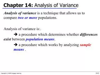
Business Statistics. Chapter 11 Analysis of Variance. Chapter Goals. After completing this chapter, you should be able to: Recognize situations in which to use analysis of variance Understand different analysis of variance designs Perform a single-factor hypothesis test and interpret results

E N D
Business Statistics Chapter 11Analysis of Variance
Chapter Goals After completing this chapter, you should be able to: • Recognize situations in which to use analysis of variance • Understand different analysis of variance designs • Perform a single-factor hypothesis test and interpret results • Conduct and interpret post-analysis of variance pairwise comparisons procedures • Set up and perform randomized blocks analysis • Analyze two-factor analysis of variance test with replications results
Chapter Overview Analysis of Variance (ANOVA) One-Way ANOVA Randomized Complete Block ANOVA Two-factor ANOVA with replication F-test F-test Tukey- Kramer test Fisher’s Least Significant Difference test
General ANOVA Setting • Investigator controls one or more independent variables • Called factors (or treatment variables) • Each factor contains two or more levels (or categories/classifications) • Observe effects on dependent variable • Response to levels of independent variable • Experimental design: the plan used to test hypothesis
One-Way Analysis of Variance • Evaluate the difference among the means of three or more populations Examples: Accident rates for 1st, 2nd, and 3rd shift Expected mileage for five brands of tires • Assumptions • Populations are normally distributed • Populations have equal variances • Samples are randomly and independently drawn
Completely Randomized Design • Experimental units (subjects) are assigned randomly to treatments • Only one factor or independent variable • With two or more treatment levels • Analyzed by • One-factor analysis of variance (one-way ANOVA) • Called a Balanced Design if all factor levels have equal sample size
Hypotheses of One-Way ANOVA • All population means are equal • i.e., no treatment effect (no variation in means among groups) • At least one population mean is different • i.e., there is a treatment effect • Does not mean that all population means are different (some pairs may be the same)
One-Factor ANOVA All Means are the same: The Null Hypothesis is True (No Treatment Effect)
One-Factor ANOVA (continued) At least one mean is different: The Null Hypothesis is NOT true (Treatment Effect is present) or
Partitioning the Variation • Total variation can be split into two parts: SST = SSB + SSW SST = Total Sum of Squares SSB = Sum of Squares Between SSW = Sum of Squares Within
Partitioning the Variation (continued) SST = SSB + SSW Total Variation = the aggregate dispersion of the individual data values across the various factor levels (SST) Between-Sample Variation = dispersion among the factor sample means (SSB) Within-Sample Variation = dispersion that exists among the data values within a particular factor level (SSW)
Commonly referred to as: Sum of Squares Within Sum of Squares Error Sum of Squares Unexplained Within Groups Variation Partition of Total Variation Total Variation (SST) Variation Due to Factor (SSB) Variation Due to Random Sampling (SSW) + = • Commonly referred to as: • Sum of Squares Between • Sum of Squares Among • Sum of Squares Explained • Among Groups Variation
Total Sum of Squares SST = SSB + SSW Where: SST = Total sum of squares k = number of populations (levels or treatments) ni = sample size from population i xij = jth measurement from population i x = grand mean (mean of all data values)
c1=c(254,263,241,237,251) • c2=c(234,218,235,227,216) • c3=c(200,222,197,206,204) • y=as.vector(rbind(c1,c2,c3)) • Use R to find mean of c1, c2, c3, y • Find deviations from the means • Find sum of squared deviations
Total Variation (continued)
Sum of Squares Between SST = SSB + SSW Where: SSB = Sum of squares between k = number of populations ni = sample size from population i xi = sample mean from population i x = grand mean (mean of all data values)
Between-Group Variation Variation Due to Differences Among Groups Mean Square Between = SSB/degrees of freedom
Between-Group Variation (continued)
Sum of Squares Within SST = SSB + SSW Where: SSW = Sum of squares within k = number of populations ni = sample size from population i xi = sample mean from population i xij = jth measurement from population i
Within-Group Variation Summing the variation within each group and then adding over all groups Mean Square Within = SSW/degrees of freedom
Within-Group Variation (continued)
One-Way ANOVA Table Source of Variation SS df MS F ratio SSB Between Samples MSB SSB k - 1 MSB = F = k - 1 MSW SSW Within Samples SSW N - k MSW = N - k SST = SSB+SSW Total N - 1 k = number of populations N = sum of the sample sizes from all populations df = degrees of freedom
One-Factor ANOVAF Test Statistic • Test statistic MSB is mean squares between variances MSW is mean squares within variances • Degrees of freedom • df1 = k – 1 (k = number of populations) • df2 = N – k (N = sum of sample sizes from all populations) H0: μ1= μ2 = …= μk HA: At least two population means are different
Interpreting One-Factor ANOVA F Statistic • The F statistic is the ratio of the between estimate of variance and the within estimate of variance • The ratio must always be positive • df1 = k -1 will typically be small • df2 = N - k will typically be large The ratio should be close to 1 if H0: μ1= μ2 = … = μk is true The ratio will be larger than 1 if H0: μ1= μ2 = … = μk is false
You want to see if three different golf clubs yield different distances. You randomly select five measurements from trials on an automated driving machine for each club. At the .05 significance level, is there a difference in mean distance? One-Factor ANOVA F Test Example Club 1Club 2Club 3 254 234 200 263 218 222 241 235 197 237 227 206 251 216 204
One-Factor ANOVA Example: Scatter Diagram Distance 270 260 250 240 230 220 210 200 190 Club 1Club 2Club 3 254 234 200 263 218 222 241 235 197 237 227 206 251 216 204 • • • • • • • • • • • • • • • 1 2 3 Club
One-Factor ANOVA Example Computations Club 1Club 2Club 3 254 234 200 263 218 222 241 235 197 237 227 206 251 216 204 x1 = 249.2 x2 = 226.0 x3 = 205.8 x = 227.0 n1 = 5 n2 = 5 n3 = 5 N = 15 k = 3 SSB = 5 [ (249.2 – 227)2 + (226 – 227)2 + (205.8 – 227)2 ] = 4716.4 SSW = (254 – 249.2)2 + (263 – 249.2)2 +…+ (204 – 205.8)2 = 1119.6 MSB = 4716.4 / (3-1) = 2358.2 MSW = 1119.6 / (15-3) = 93.3
H0: μ1 = μ2 = μ3 HA: μi not all equal = .05 df1= 2 df2 = 12 One-Factor ANOVA Example Solution Test Statistic: Decision: Conclusion: Critical Value: F = 3.885 Reject H0 at = 0.05 = .05 There is evidence that at least one μi differs from the rest 0 Do not reject H0 Reject H0 F= 25.275 F.05 = 3.885
R program c1=c(254,263,241,237,251) • c2=c(234,218,235,227,216) • c3=c(200,222,197,206,204) • f=factor(rep(1:3,5)) • y=as.vector(rbind(c1,c2,c3)) • aov(y~f); plot(f,y) #gives box plot • anova(lm(y~f)) #prints F statistic
ANOVA -- Single Factor: Excel Output EXCEL: tools | data analysis | ANOVA: single factor
The Tukey-Kramer Procedure • Tells which population means are significantly different • e.g.: μ1 = μ2μ3 • Done after rejection of equal means in ANOVA • Allows pair-wise comparisons • Compare absolute mean differences with critical range x μ μ μ = 1 2 3
Tukey-Kramer Critical Range where: q = Value from standardized range table with k and N - k degrees of freedom for the desired level of MSW = Mean Square Within ni and nj = Sample sizes from populations (levels) i and j
1. Compute absolute mean differences: The Tukey-Kramer Procedure: Example Club 1Club 2Club 3 254 234 200 263 218 222 241 235 197 237 227 206 251 216 204 2. Find the q value from the table in appendix J with k and N - k degrees of freedom for the desired level of
The Tukey-Kramer Procedure: Example 3. Compute Critical Range: 4. Compare: 5. All of the absolute mean differences are greater than critical range. Therefore there is a significant difference between each pair of means at 5% level of significance.
Randomized Complete Block ANOVA • Like One-Way ANOVA, we test for equal population means (for different factor levels, for example)... • ...but we want to control for possible variation from a second factor (with two or more levels) • Used when more than one factor may influence the value of the dependent variable, but only one is of key interest • Levels of the secondary factor are called blocks
Partitioning the Variation • Total variation can now be split into three parts: SST = SSB + SSBL + SSW SST = Total sum of squares SSB = Sum of squares between factor levels SSBL = Sum of squares between blocks SSW = Sum of squares within levels
Sum of Squares for Blocking SST = SSB + SSBL + SSW Where: k = number of levels for this factor b = number of blocks xj = sample mean from the jth block x = grand mean (mean of all data values)
Partitioning the Variation • Total variation can now be split into three parts: SST = SSB + SSBL + SSW SST and SSB are computed as they were in One-Way ANOVA SSW = SST – (SSB + SSBL)
Randomized Block ANOVA Table Source of Variation SS df MS F ratio MSBL Between Blocks SSBL b - 1 MSBL MSW Between Samples MSB SSB k - 1 MSB MSW Within Samples SSW (k–1)(b-1) MSW Total SST N - 1 k = number of populations N = sum of the sample sizes from all populations b = number of blocks df = degrees of freedom
Blocking Test • Blocking test: df1 = b - 1 df2 = (k – 1)(b – 1) MSBL F = MSW Reject H0 if F > F
Main Factor Test • Main Factor test: df1 = k - 1 df2 = (k – 1)(b – 1) MSB F = MSW Reject H0 if F > F
Fisher’s Least Significant Difference Test • To test which population means are significantly different • e.g.: μ1 = μ2≠μ3 • Done after rejection of equal means in randomized block ANOVA design • Allows pair-wise comparisons • Compare absolute mean differences with critical range x = 1 2 3
Fisher’s Least Significant Difference (LSD) Test where: t/2 = Upper-tailed value from Student’s t-distribution for /2 and (k -1)(n - 1) degrees of freedom MSW = Mean square within from ANOVA table b = number of blocks k = number of levels of the main factor
Fisher’s Least Significant Difference (LSD) Test (continued) Compare: If the absolute mean difference is greater than LSD then there is a significant difference between that pair of means at the chosen level of significance.
Two-Way ANOVA • Examines the effect of • Two or more factors of interest on the dependent variable • e.g.: Percent carbonation and line speed on soft drink bottling process • Interaction between the different levels of these two factors (only if replications exist) • e.g.: Does the effect of one particular percentage of carbonation depend on which level the line speed is set?
Two-Way ANOVA (continued) • Assumptions • Populations are normally distributed • Populations have equal variances • Independent random samples are drawn
Two-Way ANOVA Sources of Variation Two Factors of interest: A and B a = number of levels of factor A b = number of levels of factor B N = total number of observations in all cells n’= replications
Two-Way ANOVA Sources of Variation (continued) SST = SSA + SSB + SSAB + SSE Degrees of Freedom: SSA Variation due to factor A a – 1 SST Total Variation SSB Variation due to factor B b – 1 SSAB Variation due to interaction between A and B (a – 1)(b – 1) N - 1 SSE Inherent variation (Error) N – ab