Chapter 11 Analysis of Variance

1. Chapter 11Analysis of Variance 1

2. Chapter 11 Analysis of Variance 11.1 Introduction 11.2 One-Factor Analysis of Variance 11.3 Two-Factor Analysis of Variance: Introduction and Parameter Estimation 11.4 Two-Factor Analysis of Variance: Testing Hypotheses 11.5 Final Comments 2

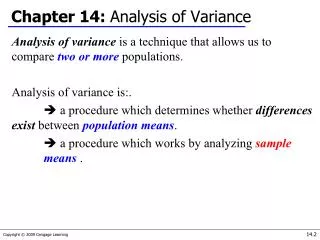
3. Introduction • When producing computer chips, the manufacturer (製造業者) needs to decide upon the raw materials (原料) to be used, the temperature at which to fuse the parts, the shape and the size of the chip, and other factors. • For a given set of choices of these factors, the manufacturer wants to know the mean quality value of the resulting chip. • This will enable her or him to determine the choices of the factors of production that would be most appropriate for obtaining a quality product. • In this chapter we introduce the statistical technique used for analyzing the foregoing type of problem. • The statistical technique was invented by R. A. Fisher and is known as the analysis of variance(ANOVA). • In all the models considered in this chapter, we assume that the data are normally distributed with the same (though unknown) variance σ2.

4. One-Factor Analysis of Variance • Consider msamples, each of size n. • Suppose that these samples are independent and that sample icomes from a population that is normally distributed with mean μiand varianceσ2, i = 1, . . . ,m. • We will be interested in testing the null hypothesis H0: μ1 = μ2 = · · · = μm against H1: not all the means are equal • We will be testing the null hypothesis that all the population means are equal against the alternative that at least two population means differ.

5. One-Factor Analysis of Variance • Note that we assume that these samples have a common varianceσ2. • How to calculate the common varianceσ2? • Method 1

6. One-Factor Analysis of Variance • Method 2

7. One-Factor Analysis of Variance • Conclusion: we can estimate σ2 by

8. One-Factor Analysis of Variance • Fact:when H0is true, TS will have what is known as an Fdistribution with m − 1 numerator (分子) and m(n − 1) denominator (分母) degrees of freedom. • Let Fm−1,m(n−1),αdenote the α critical value of this distribution. • That is, the probability that an Frandom variable having numerator and denominator degrees of freedom m − 1 and m(n − 1), respectively, will exceed Fm−1,m(n−1),α is equal to α (see Fig. 11.1). • The significance-level-α test of H0 is as follows:

9. One-Factor Analysis of Variance • Values of Fr,s,0.05 for various values of rand sare presented in App. Table D.4. • Part of this table is presented in Table 11.1. • From Table 11.1, we see that there is a 5 percent chance that an F random variable having 3 numerator and 10 denominator degrees of freedom will exceed 3.71.

10. One-Factor Analysis of Variance • A Remark on the Degrees of Freedom • The numerator degrees of freedom of the F random variable are determined by the numerator (分子) estimator . • Since is the sample variance from a sample of size m, it follows that it has m − 1 degrees of freedom. • Similarly, the denominator (分母) estimator is based on the statistic . • Since each of the sample variances is based on a sample of size n, it follows that they each have n − 1 degrees of freedom. • Summing the msample variances then results in a statistic with m(n − 1) degrees of freedom.

11. Example 11.1 • An investigator (研究者) for a consumer cooperative (消費合作社) organized a study of the mileages obtainable from three different brands of gasoline (汽油品牌). • Using 15 identical motors set to run at the same speed, the investigator randomly assigned each brand of gasoline to 5 of the motors. • Each of the motors was then run on 10 gallons of gasoline, with the total mileages obtained as follows. • Test the hypothesis that the average mileage obtained is the same for all three types of gasoline. • Use the 5 percent level of significance.

12. Example 11.1 • Solution • Since m = 3 and n = 5, the sample means are

13. Example 11.1 • Since m − 1 = 2 and m(n − 1) = 12, we must compare the value of the TS with the value of F2,12,0.05. • Now, from App. Table D.4, we see that F2,12,0.05 = 3.89. • Since the value of the test statistic (TS = 2.60) does not exceed 3.89, at the 5 percent level of significance we cannot reject the null hypothesis. • If the value of the test statistic TS is v, then the pvalue will be given by p value = P{F m−1,m(n−1) ≥ v} where F m−1,m(n−1) is an Frandom variable with m − 1 numerator and m(n − 1) denominator degrees of freedom. p value = 0.11525 (Program 11-1)

14. One-Factor Analysis of Variance

15. One-Factor Analysis of Variance • Remark • When m = 2, the preceding is a test of the null hypothesis that two independent samples, having a common population variance, have the same mean. • The reader might wonder how this compares with the one presented in Chap. 10. • It turns out that the tests are exactly the same. • That is, assuming the same data are used, they always give rise to exactly the same p value.

16. Exercise (P. 510, 1&2)

17. Exercise (P. 513, 10)

18. Two-Factor Analysis of Variance: Introduction and Parameter Estimation Example 11.3 • Four different standardized reading achievement tests were administered (實施)to each of five students. • Their scores were as follows: • Each value in this set of 20 data points is affected by two factors: the examination and the student whose score on that examination is being recorded. • The examination factor has four possible values, or levels, and the student factor has five possible levels.

19. Two-Factor Analysis of Variance: Introduction and Parameter Estimation • Let us suppose that there are mpossible levels of the first factor and npossible levels of the second. • Let Xijdenote the value of the data obtained when the first factor is at level iand the second factor is at level j. • Recall Sec. 11.2. Let Xijrepresent the value of the jth member of sample i. where αiequal to the deviation of μi fromthe average of the means μ.

20. Two-Factor Analysis of Variance: Introduction and Parameter Estimation • In the case of two factors, we write our model in terms of row and column deviations. • The value μ is referred to as the grand mean, αi is the deviation from the grand mean due to row i, and βjis the deviation from the grand mean due to column j. • “Dot” notation

21. Two-Factor Analysis of Variance: Introduction and Parameter Estimation • To determine estimators for parameters μ, αi,and βj, i = 1, . . . ,m, j = 1, . . . , n. (“Dot” notation)

22. Example 11.4 • The following data from Example 11.3 give the scores obtained when four different reading tests were given to each of five students. • Use it to estimate the parameters of the model.

23. Example 11.4 • Therefore, for instance, if one of the students is randomly chosen and then given a randomly chosen examination, then our estimate of the mean score that will be obtained is . • If we were told that examination i was taken, then this would increase our estimate of the mean score by the amount . • If we were told that the student chosen was number j, then this would increase our estimate of the mean score by the amount . • Thus, for instance, we would estimate that the score obtained on examination 1 by student 2 is the value of a random variable whose mean is

24. Exercise (P. 519, 4)

25. Exercise (P. 519, 3)

26. Two-Factor Analysis of Variance: Testing Hypotheses • Consider the two-factor model in which one has data values Xij, i = 1, . . . ,m andj =1, . . . , n. • These data are assumed to be independent normal random variables with a common variance σ2 and with mean values satisfying where • In this section, we will test • Here we will apply the analysis of variance approach in which twodifferent estimators are derived for the variance σ2. • The first will always be a valid estimator, whereas the second will be a valid estimator only when the null hypothesis is true.

27. Two-Factor Analysis of Variance: Testing Hypotheses • Method 1 (estimate variance σ2) • The sum of the squares of Nstandard normal random variables is a chi-squared random variable with Ndegrees of freedom.

28. Ch. 7 Distribution of the Sample Variance of a Normal Population

29. Ch. 7 Distribution of the Sample Variance of a Normal Population

30. Two-Factor Analysis of Variance: Testing Hypotheses • Since

31. Two-Factor Analysis of Variance: Testing Hypotheses

32. Two-Factor Analysis of Variance: Testing Hypotheses • Method 2 (estimate variance σ2) • Suppose we want to test the null hypothesis that there is no row effect • Note that when H0 is true, each αiis equal to 0, and • Since each Xi. is the average of n random variables with varianceσ2 • When H0 is true, will be chi squared with mdegrees of freedom.

33. Two-Factor Analysis of Variance: Testing Hypotheses • When H0 is true, • It can be shown that SSr/(m − 1) will tend to be larger than σ2 when H0 is not true.

34. Two-Factor Analysis of Variance: Testing Hypotheses • The test of the null hypothesis H0 that there is no row effect involves comparing the two estimators just given, and it calls for rejection when the second is significantly larger than the first. • The test statistic • The significance-level-αtest is • If the value of the test statistic is v, then the pvalue where Fm−1,N is an F random variable with m−1numerator and N denominator degrees of freedom.

35. Two-Factor Analysis of Variance: Testing Hypotheses

36. Example 11.5 • The following are the numbers of defective items produced by four workers using, in turn, three different machines. • Test whether there are significant differences between the machines and the workers. • Solution • Here m = 3 and n = 4, computing the row and column averages:

37. Example 11.5 • The calculation of SSeis more involved because we must add the sum of the squares of the terms Xij−Xi.−X.j+X..as i ranges from1to 3 and j from1to 4. For example, • Adding all 12 terms gives

38. Example 11.5 • Since m−1=2 and N=2·3=6, the test statistic for the hypothesis that there is no row effect is • From App. Table D.4 we see that F2,6,0.05 = 5.14, and so the hypothesis that the mean number of defective items is unaffected by which machine is used is not rejected at the 5 percent level of significance. • The test statistic for the hypothesis that there is no column effect is • From App. Table D.4 we see that F3,6,0.05 = 4.76, and so the hypothesis that the mean number of defective items is unaffected by which worker is used is also not rejected at the 5 percent level of significance.

39. Example 11.5 • Running Result of Program 11-2 • The value of the F-statistic for testing that there is no row effect is 1.2127 • The p-value for testing that there is no row effect is 0.3571 • The value of the F-statistic for testing that there is no column effect is 0.4042 • The p-value for testing that there is no column effect is 0.7555

40. Exercise (P527, 1)

41. KEY TERMS • One-factor analysis of variance: A model concerning a collection of normal random variables. It supposes that the variances of these random variables are equal and that their mean values depend on only a single factor, namely, the sample to which the random variable belongs. • F statistic: A test statistic that is, when the null hypothesis is true, a ratio of two estimators of a common variance. • Two-factor analysis of variance: A model in which a set of normal random variables having a common variance is arranged in an array of rows and columns. The mean value of any of them depends on two factors, namely, the row and the column in which the variable lies. 41