Download
1 / 43
430 likes | 459 Vues
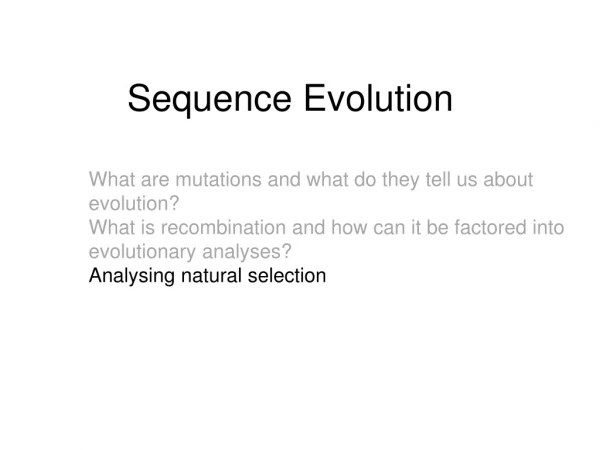
Sequence Evolution. What are mutations and what do they tell us about evolution? What is recombination and how can it be factored into evolutionary analyses? Analysing natural selection. A. T. A. T. What are mutations?. G. C. G. C. Chemicals Light High energy particles. T. A. T.

E N D
Sequence Evolution What are mutations and what do they tell us about evolution? What is recombination and how can it be factored into evolutionary analyses? Analysing natural selection
A T A T What are mutations? G C G C Chemicals Light High energy particles T A T A G C T A C G C G C G C G
Diverse swarm of up to1012 unique genomes within an infected individual Consensus/average sequence at centre of swarm Why are mutations important? eg. An HIV infection as a microcosm of species evolution on earth Error prone replication First HIV genome Almost all HIV genomes in an infected individual are unique All single,alldoubleand mosttriplenucleotide mutants exist/have existed within the swarm. Every possible drug resistanceand immune evasionmutation exists BEFORE any drug or immune pressures are exerted. There may be more genomic diversity within one swarm than exists within entire species of higher organisms
Neutral Harmful Potentially useful mutations may have no immediate value and might only be beneficial under certain circumstances Most non-neutral mutations will be harmful Useful mutations will occur in genomes that contain mutations that are harmful. The Problem With Mutation 4 types of mutant Conditionally useful Useful
The survival of mutations more common more useful less useful Frequency of a mutation in the population Rate of fixation is proportional to how useful the mutation is less common Time since the mutation arose In big populations useful mutations generally get “fixed” and harmful ones do not
The survival of mutations Fixation = when the mutant becomes the wild-type more common Rate of loss is proportional to how harmful the mutations are Frequency of a mutation in the population more harmful less harmful less common Time since the mutation arose In big populations useful mutations generally get “fixed” and harmful ones do not
The survival of mutations more common Some useful and conditionally-useful mutations never reach fixation This pattern can be caused by something called balancing selection Frequency of a mutation in the population less common Time since the mutation arose Eg mutations causing sickle cell anaemia (which is usually harmful) also provide resistance to malaria
Looking at it from a sequence perspective ACGTACGT ACGTACGT ACGTACGT ACGTACGT ACGTACGT A constant population with only 5 clonal individuals (i.e. they are all genetically identical)
Looking at it from a sequence perspective ACGTACGT GCGTACGT Replication errors introduce mutations – Harmful, useful, conditionally useful and neutral ACGTACGT ACGCACGT ACGTACGT ACGTATGT ACGTACGT ACGTACGC ACGTACGT ACAAACGT Some individuals reproduce others don’t but always the population size stays the same
Looking at it from a sequence perspective ACGTACGT GCGTACGT ACGCACAT ACGTACGT ACGCACGT ACGCACGC ACGTACGT ACGTATGT ACGCGCGT ACGTACGT ACGTACGC CCGTACGC ACGTACGT ACAAACGT ACGTACGC Fitter individuals generally produce more offspring than less fit ones
Phylogenetic trees ACGTACGT GCGTACGT ACGCACAT ACGCACAT ACGTACGT ACGCACGT ACGCACGC AGGCGCGT ACGTACGT ACGTATGT ACGCGCGT ACGCGCGT ACGTACGT ACGTACGC CCGTACGC CCGTACGC ACGTACGT ACAAACGT ACGTACGC CCCTACGC If you sample just these sequences is it possible to work out the evolutionary relatedness of the sequences
Phylogenetic trees ACGTACGT GCGTACGT ACGCACAT ACGCACAT ACGCACGT ACGCACGC AGGCGCGT ACGTACGT ACGTATGT ACGCGCGT ACGCGCGT ACGTACGT ACGTACGC CCGTACGC CCGTACGC ACGTACGT ACGTACGT ACAAACGT ACGTACGC CCCTACGC Is it possible to retrace this route?
A simple method 1 vs 2 = 3 1 vs 3 = 3 1 vs 4 = 4 1 vs 5 = 5 2 vs 3 = 1 2 vs 4 = 5 2 vs 5 = 6 3 vs 4 = 4 3 vs 5 = 5 4 vs 5 = 1 ACGCACAT 1 AGGCGCGT 2 ACGCGCGT 3 CCGTACGC 4 CCCTACGC 5 Step 1 count the number of differences between each pair of sequences
A simple method 1 vs 2 = 3 1 vs 3 = 3 1 vs 4 = 4 1 vs 5 = 5 2 vs 3 = 1 2 vs 4 = 5 2 vs 5 = 6 3 vs 4 = 4 3 vs 5 = 5 4 vs 5 = 1 1 2 3 4 5 ACGCACAT 1 1 - 3 3 4 5 AGGCGCGT 2 2 3 - 1 5 6 ACGCGCGT 3 3 3 1 - 4 5 CCGTACGC 4 CCCTACGC 5 4 4 5 4 - 1 5 5 6 5 1 - Step 1 It helps if you put these into a table (called a distance matrix)
A simple method 1 vs 2 = 3 1 vs 3 = 3 1 vs 4 = 4 1 vs 5 = 5 2 vs 3 = 1 2 vs 4 = 5 2 vs 5 = 6 3 vs 4 = 4 3 vs 5 = 5 4 vs 5 = 1 1 2 3 4 5 ACGCACAT 1 1 - 3 3 4 5 AGGCGCGT 2 2 3 - 1 5 6 ACGCGCGT 3 3 3 1 - 4 5 CCGTACGC 4 CCCTACGC 5 4 4 5 4 - 1 5 5 6 5 1 - Step 2: Find the lowest number in the table – this indicates the sequence pair with the shortest genetic distance
A simple method 1 vs 2 = 3 1 vs 3 = 3 1 vs 4 = 4 1 vs 5 = 5 2 vs 3 = 1 2 vs 4 = 5 2 vs 5 = 6 3 vs 4 = 4 3 vs 5 = 5 4 vs 5 = 1 1 2 3 4 5 ACGCACAT 1 1 - 3 3 4 5 AGGCGCGT 2 2 3 - 1 5 6 ACGCGCGT 3 3 3 1 - 4 5 CCGTACGC 4 CCCTACGC 5 4 4 5 4 - 1 5 5 6 5 1 - Step 2: 2 pairs (2 vs 3 and 4 vs 5) are tid for the smallest genetic distances
A simple method 1 vs 2 = 3 1 vs 3 = 3 1 vs 4 = 4 1 vs 5 = 5 2 vs 3 = 1 2 vs 4 = 5 2 vs 5 = 6 3 vs 4 = 4 3 vs 5 = 5 4 vs 5 = 1 1 2 3 4 5 ACGCACAT 1 1 - 3 3 4 5 AGGCGCGT 2 2 3 - 1 5 6 ACGCGCGT 3 3 3 1 - 4 5 CCGTACGC 4 CCCTACGC 5 4 4 5 4 - 1 5 5 6 5 1 - Step 2: Just choose one – it doesn’t matter which
A simple method 1 2 3 4 5 2 1 - 3 3 4 5 3 2 3 - 1 5 6 3 3 1 - 4 5 4 4 5 4 - 1 5 5 6 5 1 - = a distance of 0.5 Step 2: here we choose 2 vs 3 – and use these to start our tree.
A simple method 1 2 3 4 5 2 1 - 3 3 4 5 3 2 3 - 1 5 6 3 3 1 - 4 5 4 4 5 4 - 1 5 5 6 5 1 - = a distance of 0.5 Step 2: the genetic distance between 3 and 2 is proportional to the length of the branch separating them (in this case 0.5 + 0.5 = 1) .
A simple method 1 2 3 4 5 2/3 2 1 - 3 3 4 5 3 2 3 - 1 5 6 3 3 1 - 4 5 4 4 5 4 - 1 5 5 6 5 1 - = a distance of 0.5 Step 3: Now merge the distances of sequences 2 & 3 to get the distances between the “node” (i.e. the red spot labelled 2/3) and the other three sequences.
A simple method 1 2/3 4 5 2/3 2 1 - 3 4 5 3 2/3 3 - 4.5 5.5 4 4 4.5 - 1 5 5 5.5 1 - = a distance of 0.5 Step 3: Now merge the distances of sequences 2 & 3 to get the distances between the “node” (i.e. the red spot) and the other three sequences.
A simple method 1 2/3 4 5 2/3 2 1 - 3 4 5 3 2/3 3 - 4.5 5.5 4 4 4.5 - 1 5 5 5.5 1 - = a distance of 0.5 Step 3: Now repeat from step 2.
A simple method 1 2/3 4 5 2/3 2 1 - 3 4 5 3 2/3 3 - 4.5 5.5 4/5 4 4 4 4.5 - 1 5 5 5.5 1 - 5 = a distance of 0.5 Step 2: Choose shortest distance ( 4 vs 5) and add this to the tree.
A simple method 1 2/3 4/5 2/3 2 1 - 3 4.5 3 2/3 3 - 5 4/5 4 4/5 4.5 5 - 5 = a distance of 0.5 Step 3: Merge(4 vs 5) and return to step 2.
A simple method 1 1 2/3 4/5 1/2/3 2/3 2 1 - 3 4.5 3 2/3 3 - 5 4/5 4 4/5 4.5 5 - 5 = a distance of 0.5 Step 2: Find next smallest (1 vs 2/3) and add these to the tree.
A simple method 1 1/2/3 1/2/3 4/5 2/3 2 1/2/3 - 4.75 3 - 4/5 4.75 4/5 4 5 = a distance of 0.5 Step 3: Merge(1/2/3) and add go back to step 2.
A simple method 1 1/2/3 1/2/3 4/5 2/3 2 1/2/3 - 4.75 1/2/3/4/5 3 - 4/5 4.75 4/5 4 5 = a distance of 0.5 Step 2: only one pair left (1/2/3 vs 4/5) so pick these and join them up to finish the tree.
A simple method 1 1/2/3 1/2/3 4/5 2/3 2 1/2/3 - 4.75 1/2/3/4/5 3 - 4/5 4.75 4/5 4 5 = a distance of 0.5 If you go back and check you will see that this is the correct tree
Interpreting trees 1 1 2 2 = 3 3 4 4 5 5
The direction of evolution in un-rooted trees is not always obvious Rooting 1 1 2 2 = 3 3 4 4 5 5 = root (node representing the most recent common ancestor) = direction of evolution
The direction of evolution in un-rooted trees can be really hard to determine if the root position is unknown Rooting 1 1 2 2 = 3 3 4 4 5 5 5 = root = direction of evolution
Rooted trees are better than unrootedtrees The direction of evolution in rooted trees is obvious 1 1 2 2 ~ 3 3 4 4 5 5 “Outgroup” An outgroup = one or more sequences that are more distantly related to the sequences of interest than the sequences of interest are to one another
Other methods of making trees This tree is called an “UPGMA dendrogram” 1 1/2/3 2/3 2 1/2/3/4/5 3 4/5 4 5
Other methods of making trees Others are: Neighbour joining Least squares Maximum parsimony Maximum likelihood Bayesian 1 1/2/3 2/3 2 1/2/3/4/5 3 4/5 4 5
Other methods of making trees There are lots of free computer programs that will make these trees for you (ones in red are easy to use and will display the trees for you) Neighbour joining – Mega, RDP, PAUP, PHYLIP Least squares – RDP, PHYLIP Maximum parsimony – Mega, PHYLIP, PAUP Maximum likelihood – Mega,RDP, RAXML, PHYML Bayesian – RDP, MrBAYES, BEAST Less sophisticated More sophisticated
Other methods of making trees There are lots of free computer programs that will make these trees for you (ones in red are easy to use and will display the trees for you) Neighbour joining Least squares Maximum parsimony Maximum likelihood Bayesian MCMC Less sophisticated Like UPGMA these methods use distance matrices. LS is slightly more accurate but NJ is MUCH faster More sophisticated
Other methods of making trees There are lots of free computer programs that will make these trees for you (ones in red are easy to use and will display the trees for you) Neighbour joining Least squares Maximum parsimony Maximum likelihood Bayesian MCMC Less sophisticated These methods examine the actual nucleotide substitutions. MP and newer ML methods are reasonably fast but much slower & computationally intensive BMCMC methods if used properly are generally more accurate More sophisticated
Other methods of making trees There are lots of free computer programs that will make these trees for you (ones in red are easy to use and will display the trees for you) Neighbour joining Least squares Maximum parsimony Maximum likelihood Bayesian MCMC Less sophisticated ML and BMCMC methods can apply complex evolutionary models during tree inferance More sophisticated
Models of evolution Nucleotide substitution Amino acid substitution Demographic Molecular clock Phylogeographic Jukes Cantor (JC) – all types of nucleotide substitution are equally likely Kimura 2 parameter (K2P) – transitions and transversions are not equally likely General time reversible (GTR/REV) – the six reversible substitution types can all occur at different rates Both ML and BMCMC methods can apply these
Models of evolution Nucleotide substitution Amino acid substitution Demographic Molecular clock Phylogeographic Codon models – in coding regions 1st 2nd and 3rdcodon positions can all have different substituton rates. Both ML and BMCMC methods can apply these
Models of evolution Nucleotide substitution Amino acid substitution Demographic Molecular clock Phylogeographic Exponential variation in population size – population sizes can remain constant or increase at a constant rate Bayesian skyline plot (BSP) – rates of population size increase/decrease can vary over time. Only some of the BMCMC methods can apply these
Models of evolution Nucleotide substitution Amino acid substitution Demographic Molecular clock Phylogeographic Strict clock – rates of nucleotide substitution remain constant during evolution Relaxed clock – rates of nucleotide substitution are free to vary through time and from one lineage to the next Only some of the BMCMC methods can apply these and sequence sampling dates must be supplied
Models of evolution Nucleotide substitution Amino acid substitution Demographic Molecular clock Phylogeographic Constant diffusion rates – rates of movement remain constant during evolution Relaxed diffusion rates – rates of movement are free to vary through time and from one lineage to the next Discrete diffusion – movement between discrete locations is modelled (eg from country to country) Continuous diffusion – Eg movement is modelled over a continuous surface (eg using GPS coordinates) Only some of the BMCMC methods can apply these and sequence sampling locations must be supplied