Download
1 / 15
150 likes | 303 Vues
Topics in Random Processes. CSE 5301 – Data Modeling Guest Lecture: Dr. Gergely Z á ruba. Poission Process. The Poission process is very hand when modeling birth/death processes, like arrival of calls to a telephone system.

E N D
Topics in Random Processes CSE 5301 – Data Modeling Guest Lecture: Dr. Gergely Záruba
Poission Process • The Poission process is very hand when modeling birth/death processes, like arrival of calls to a telephone system. • We can approach this by discretizing time, and assuming that in any time slot an event is happening with probability p. However two events cannot happen in the same time slot. Thus we need to reduce the size of the time slots to infinitesimally small slots. • Thus, we need to talk about the rate (events/time). • Number of events in a given time duration is thus Poisson distributed • The time between consecutive events (inter-arrival time) is inverse-exponentially distributed.
Heavy Tails • A pdf is a function that is non-negative and for which the indefinit integral is 1. • We have looked at pdf-s that decay exponentially (e.g., gaussian, inverse-exponential) • Can we create a pdf-like function that decays like 1/x ? - Although the function converges to 0, the integral of the function has a logarithmic flavor and thus will never integrate to 1. • Can we create a pdf-like function that decays like x^-2? - The integral of the function has 1/x flavor and thus can work as a pdf. However, when calculating the mean the integral turns the function again to a divergent function. Thus this pdf has an infinite mean. • Similarly, we can see, that a x^-3 like decay can result in a pdf with a finite mean but infinite variance. • These latter two pdfs are good examples of heavy tailed distributions! Unfortunately, many processes have heavy-tailed features.
Heavy Tail’s Impact on CLT • For the Central Limit Theorem to work, the distributions from which the random numbers added are generated have to have finite means and variances. • Thus, if the underlying distribution from which the samples come is heavy tailed, then we cannot use significance testing and confidence intervals. • Unfortunately, it has been shown that Internet traffic can be modeled by a Pareto distribution most closely. Thus if traffic is modeled this way, then significance of results cannot be established.
Random Numbers in Computers • Truly random numbers in proper digital logic do not exist. • We can use algorithms that generate sequences of numbers that have statistical properties as if they were generated by a uniform distribution. • Pseudo-random and quazi-random number generators. • Pseudo-random number generators generate a random looking integer between 1 and MAX_RAND. • They are actually sequences of numbers, where the seed is is the first number in the series. • This lack of randomness is actually great for computer simulations: our experiments can be repeated deterministically. We set the seed usually once at the beginning. Different experiments are created by setting different seeds.
Random Variate Generation • So, we can generate uniform random numbers. By dividing by MAX_RAND we have a semi-continous random between (0,1). • How can we use this to generate random numbers of different distributions? • We need to obtain the cdf of the distribution and invert it. Then substituting the (0,1) uniform random into the inverse cdf we get the properly distributed random number. • As an example, the inverse exponential distribution’s inverse cdf is: -log(1-u)/lambda (where u is the (0,1) random)
How about Generating Normal? • Unfortunately, the normal distribution does not have a closed form for its inverse cdf (and the normal is not the only such distribution) • We could sum up a large number (>30) of uniform randoms and scale it to the proper mean and variance. • There are other approximations, usually based on trigonometric functions.
Resolution of Random Numbers and Their Impact • When we create rand()/MAX_RAND, we end up with a floating point number. However not only is this number a rational number (we cannot have irrational numbers in computers), its values are never closer than 1/MAX_RAND. • Thus, when substituting into the inverse cdf, the shape of the inverse cdf will determine how close the final random variates’ values will be. • This is especially significant of a problem for heavy tailed distributions, where theoretically there are larger chances to create very small or very large numbers, which may be prohibited from generation by the resolution of the (0,1) random.
Case Study: Aloha • The Aloha networking protocol was used to connect computers distributed over the Hawaiian islands with a shared bandwidth wireless network. • The medium (the radio bandwidth) had to be shared by many radios. The task is to come up with effective and fair ways to share. • Aloha was the first approach and it is characterized by the lack of an approach. As soon as data is ready to be transmitted, a radio node is going to transmit it. • This is a straight forward application of a Poission process.
Case Study: Aloha • Let us assume, that any time a node transmits, it is going to transmit for T duration. Let us assume that the arrival of this transmission events follows a Poission process (it is a straight forward assumption). • Let us assume that a node starts transmitting at time t0. In order for this to be successful, no other node should transmit in the time period (t0-T,t0+T), i.e., the collision domain is 2*T. • What is the utilization of this network? • The rate of arrival is l. This is our best guess (the mean of the Poisson) of how many arrivals happen in a time frame. • What I then the probability that none of the other nodes transmit for 2T duration? It is a Poisson with (2T,0).
Case Study: Aloha • Thus it is: l^0 * e^(-2l) / 0! Which is e^-2l • Thus the total utilization is: l*e^-2l • After differentiating this we will find its maximum to be at l=0.5 where the value is 1/(2e)= 18% • This is not great. • We can easily double the performance by synchronizing the network (slotted-Aloha) and making sure that nodes can only start transmitting at time instances that are integer multiples of T.
Revisiting Confidence Intervals • We have a random process that generates random numbers with an underlying mean m and standard deviation s . • We take N samples. Based on this N samples we can calculate the sample mean m and unbiased sample standard deviation s. • We want to claim a C% confidence (e.g., C=0.95) • We want to say something about the relationships of m and m, more precisely we want the Pr(m-e< m <m+e)>C • The interval (m-e,m+e) is our confidence interval • The error e is: e= z(a)*s/N if we have taken enough samples (N>30) or if we know that the underlying distribution is Gaussian. (otherwise, we have to calculate with t(a,N) ). z(a) is the a-th percentile of the standard normal (e.g., for a 95% confidence it would be 1.96)
Being Confident the Relative Way • Unlike social science statisticians, using computer simulations we usually do not have a limit on our sample size. We can always run more simulations (time permitting) with different seeds. • We can draw our data points in figures with confidence bars over them, but this can result in messy figures. • Sometimes it is better to just show our best estimate but making sure that we bound the error. • Thus we can talk about figures having a confidence value and bound relative errors. Our relative error is the error e divided by the best guess m. er=e/m • We should run enough simulations (large enough N) to claim a large confidence that our relative error is less than a small number (in engineering 95% confidence with 5% relative error is usually an acceptable minimum)
Being Confident; the Recipe • Make sure that simulation does not model heavy tailed distributions and that you have an argument that the underlying random variable has a finite mean ad variance. • Set N0=30 (if you do not know that the underlying is a Gaussian) • Run the simulation N0 times with N0 different seeds. • Calculate the mean m0, the standard deviation s0, the error e0, and the relative error er0 based on a chosen confidence level C. If er0 less than the target relative error ert(e.g., 5%) then you are done with the data point. • If not, you need to estimate how many simulation runs you need to be confident. This can be done based on the current data. Assume that the mean and the standard deviation are not going to change to the worse, then you can calculate the target error (et0< m0 * ert). • Turning the error’s function around: N= (z(a)*s/e)^2 we can estimate the number of samples needed by: N1= (z(a)*s0/et0)^2 • Throw out the data points, chose N1 different seeds (different than before) and repeat the experiment from bullet point 3. Iterate as long as bullet point 4 checks out (which is likely going to be your second iteration).
Case Study: Aloha, a Simulation • Look at the main code in the Aloha simulation example. • The code corresponds to the previous recipe. • Try to enter simulation parameters that will not result in confidence after 30 runs.