Imputing species-level plot basal area and tree density attributes from remotely sensed data in north-central Idaho

1. Imputing species-level plot basal area and tree density attributes from remotely sensed data in north-central Idaho Andrew T. Hudak Nicholas L. Crookston Jeffrey S. Evans Rocky Mountain Research Station Moscow. Idaho

2. Location map of the Moscow Mountain and St. Joe Woodlands lidar study areas Hudak et al., CJRS 32:126-138.

3. Hudak et al., CJRS 32:126-138.

4. Hudak et al., CJRS 32:126-138.

5. Scatterplots of predictions versus observations (N = 165) for ln-transformed a) basal area and b) tree density and natural scale c) basal area and d) tree density (lines indicate 1:1 relationship; “∆” = Moscow Mountain plots; “+” = St. Joe Woodlands plots) Hudak et al., CJRS 32:126-138.

6. Objective: Impute plot-level Y variables (available at limited, discrete locations) using pixel-level, remotely sensed X variables (available globally) Why? So we can map Y variables of interest

7. Lidar acquired summer 2003; 55,000 ha 81 plots, 2003 & 2004 field seasons Lidar acquired summer 2003; 32,000 ha 84 plots, 2003 & 2004 field seasons

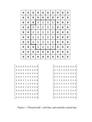
8. Sampling and Scaling Issues Y variables measured at plot scales: 1/10 acre (Moscow Mt.) = 405 m2 1/5 acre (St. Joe) = 810 m2 X variables measured at pixel scales: 1 m x 1 m = 1 m2 2 m x 2 m = 4 m2 6 m x 6 m = 36 m2 10 m x 10 m = 100 m2 30 m x 30 m = 900 m2 Regardless of resolution, values of pixels intersecting the plot footprint were averaged.

9. NA NA NA Conifer Species Basal Area Summarized per Study Area

10. NA NA NA Conifer Species Tree Density Summarized per Study Area

11. Basal Area (m2/ha) Tree Density (trees/ha) PIPO_BA PIPO_TD Pinus ponderosa PSME_BA PSME_TD Pseudotsuga menziesii LAOC_BA LAOC_TD Larix occidentalis PICO_BA PICO_TD Pinus contorta ABGR_BA ABGR_TD Abies grandis THPL_BA THPL_TD Thuja plicata TSHE_BA TSHE_TD Tsuga heterophylla PIEN_BA PIEN_TD Picea engelmannii ABLA_BA ABLA_TD Abies lasiocarpa Total_BA Total_TD Total (all species) warm/dry cool/wet Y variable summary: Conifer species selected (N=20) from tree species sampled (N=34) in field plots (N=165) Conifer species

12. X variable summary: Remotely sensed variables selected (N=37) from candidate remotely sensed variables (N=54) with global coverage

13. Tested statistical methods for finding nearest neighbors

14. Observed vs. Imputed values, Y variables (N=20) Pearson correlation (r) Imputation Method

15. Observed vs. Imputed values, Y variables (N=20) Root Mean Squared Difference (RMSD) Imputation Method

16. k=6 nearest neighbors, inverse distance weighted k=1 nearest neighbor RMSD RMSD k=6 nearest neighbors, inverse distance weighted k=1 nearest neighbor r r

17. Histograms of Observed and Imputed values Imputed Values = Closest Nearest Neighbor

18. Histograms of Observed and Imputed values Imputed Values = Mean of 6 Nearest Neighbors, Inverse Distance-Weighted

19. Histograms of Observed and Imputed values Imputed Values = Mean of 6 Nearest Neighbors

20. Histograms of Observed and Imputed values Imputed Values = Closest Nearest Neighbor

29. Conclusions • Choice of statistics to use for evaluating imputation results is important and remains challenging • Advantage of improved correlation and RMSD statistics by imputing from k>1nearest neighbors may be outweighed by disadvantage of an altered distribution of imputed values relative to observed values • Random Forest may provide more analytical flexibility, robustness, and predictive power than traditional imputation methods

30. Acknowledgments • Funding: • Agenda 2020 Program • Rocky Mountain Research Station • Industry Partners: • Potlatch, Inc. • Bennett Lumber Products, Inc.

31. Candidate X variables (N=54) calculated from pixel data within plot footprints

32. Candidate X variables (N=54) calculated from pixel data within plot footprints Selected X variables (N=37)