Download
1 / 24
240 likes | 319 Vues
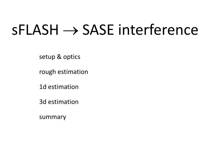
sFLASH SASE interference. s etup & optics. rough estimation. 1d estimation. 3d estimation. summary. s etup & optics. from. e stimated electron beam properties. E 585 MeV. E rms 150 k eV. n 1.5 µm. q 0.3 nC. I peak 1.5 k C. e stimated photon beam properties.

E N D
sFLASH SASE interference setup & optics rough estimation 1d estimation 3d estimation summary
setup & optics from
estimated electron beam properties E 585 MeV Erms 150 keV n 1.5 µm q 0.3 nC Ipeak 1.5 kC estimated photon beam properties modulator undulator K = 4.3 L = 1.45 m
modulation amplitude undulator FLASH @ 19 nm laser
x / m y/ m vertical correctors quads undulators chicane 1 chicane 2 chicane 3
rough estimation 1 2 (1) - energy modulation (2) - conversion to density modulation, chicane 1, r56c1 = 220 µm (saturation)
if linear: 2 3 4 (23) - discrete impedance, L 23 m, av 10 m from 15 amplification of energy modulation (3) - chicane 1, r56c3 = 170 µm 10 amplification of density modulation (34) - discrete impedance, L 16 m, av 10 m
1d estimation 1 2 3 4 5 1 discrete modulation 12 discrete impedance, L = 2.6 m, av = 10.6 m 2 discrete longitudinal dispersion, chicane 1, r56 = 220 µm 23 discrete impedance, L = 4.7 m, av = 10.1 m 3discrete longitudinal dispersion, chicane 2, r56 = 3µm 34 discrete impedance, L = 17.7 m, av = 7.7 m 4discrete longitudinal dispersion, chicane 3, r56 = 170 µm 45 discrete impedance , L = 16.3 m, av = 9.8 m
1d estimation 40E6 macro particles energy modulation: discrete in middle of modulator space charge interaction: discrete, 1d no CSR interaction next slide: explore linear domain initial modulation amplitude initial uncorrelated energy spread
longitudinal phase space current
MeV MeV non linear !!! ~ 3 MeV rms energy spread
MeV MeV non linear !!! ~ 3.5 MeV rms energy spread
~ 3.5 MeV rms energy spread 3D ~ 2 MeV rms
3d estimation 20E6 macro particles modulation: Emod = 250 keV discrete in middle of modulator (= instantaneous) space charge interaction: full 3d Poisson solver equidistant mesh: 15 µm × 15 µm × 800 nm/(10) step width: 2 cm (beam-line coordinate) no CSR interaction
3D Calculation Emod = 250 keV current bunch coordinate / m beam line coordinate / m
3D Calculation ~ 2.5 m Emod = 250 keV after chicane 1 before chicane 2 Current / A rms spread in 400 nm “slice” rms spread in 400 nm “slice” _rms / eV / eV bunch coordinate / m
3D Calculation ~ 14.6 m Emod = 250 keV after chicane 2 before chicane 3 Current / A rms spread in 400 nm “slice” rms spread in 400 nm “slice” _rms / eV / eV bunch coordinate / m
3D Calculation ~ 14.2 m Emod = 250 keV after chicane 3 before SASE undulator Current / A 50 µm, 170 fsec rms spread in 400 nm “slice” rms spread in 400 nm “slice” _rms / eV ~ 2 MeV rms 15 µm, 50 fsec / eV bunch coordinate / m
3D Calculation Emod = 250 keV current / A bunch coordinate 1E-4 / m beam line coordinate / m
current/A beam line coordinate/ m bunch coordinate/ m “side view” current/A period of plasma oscillation 120 m beam line coordinate/ m
summary modulator: 1d estimation (without plasma osc.): linear gain ~ 100 saturation even with minimal modulation 3d estimation: plasma oscillations, period 120 m gain length (Ming Xie) weak amplification in 30 m SASE undulator
First Shot at Statistics • Assume laser pulse eliminates lasing within FWHM completely • Take a few hundred SASE simulation results (0.25 nC) and apply the above • Let the ‘laser pulse’ jitter by about 100 fs
Comparison to Observation The rough estimate Observed behavior Energy in photon pulse Electron macro pulse number


![G4 - AMATEUR RADIO PRACTICES [5 Questions - 5 groups]](https://cdn2.slideserve.com/4809344/g4-amateur-radio-practices-5-questions-5-groups-dt.jpg)