Download
1 / 46
460 likes | 552 Vues
Ensembling Medium Range Forecast MOS GUIANCE. By Richard H. Grumm National Weather Service State College PA 16803 and Robert Hart The Florida State University. Introduction. Model Output Statistics (MOS) Regression equations of parameters from models to make a forecast for a point.

E N D
Ensembling Medium Range Forecast MOS GUIANCE By Richard H. Grumm National Weather Service State College PA 16803 and Robert Hart The Florida State University
Introduction • Model Output Statistics (MOS) • Regression equations of parameters from models to make a forecast for a point. • statistical equations were specifically tailored for each location, taking into account factors such as local climate. • MOS equations are based on output from a single model • Models have bias and errors • This will affect, though some statistical corrections, the MOS output • Timing errors andintensity errors will affect the outcome
Introduction-II • Verification Issues • Base line the extended MOS and ENSEMBLE of extended MOS with more widely used products • FWC- NGM based MOS • MET – Eta based MOS • MAV – GFS based MOS • Limited at this time to temperatures only • Average (bias or avg), Mean Absolute Error (MAE) and root-mean square error (RMSE). • Primary Goal is to evaluate the longer term MOS guidance and an Ensemble • But the shorter term MOS helps illustrate the point • Helps us further learn about ensembles and ensemble strategies.
Medium Range Forecast MOS • Produced from data from the Global forecast system (GFS) at the highest resolution of the model • Known as the Extended Range GFS MOS (MEX) • Message contains routine variables and a climate range of data at some locations at the end of the message • Most widely used extended range MOS product • Based on the highest resolution forecast model
MEX Ensemble MOS • NCEP runs the GFS and has an GFS ensemble prediction system (EPS) • MOS is generated for each GFS EPS member • The control run is slightly coarser resolution than the operational GFS • The control is used to produce perturbed members • There are 5 positive (P1-P5) • and 5 negatively (N1-N5) perturbed members based on the control run • This provides 12 GFS runs to produce MEX guidance • the operational MRF MOS prediction equations are applied to the output from each of the ensemble runs
Why Ensemble MOS? • The operation GFS and its MOS • are expected to be more accurate • Due to higher resolution which we expect to be more accurate • But may pay for timing and intensity errors as finer scale systems typically correlate less in space. • The ENSEMBLE of the MOS…. • Will show a range and times of high disagreement ~ UNCERTAINTY
Ensembles help usquick review of ensemble concepts • Deal with uncertainties in data (initial conditions) • the ability to properly resolve the feature • Deal with uncertainties in data verse resolution of the model • 6D rule, we may under sample a system. • Deal with uncertainties in physics • Current GFS system is based solely on the same model • Only variation is initial conditions
Envelope of solutions at single time Solution Forecasts Initialized at most recent data time Forecast Length GFS EPS with varied initial Conditions
Displaying uncertainties in forecasts • In Model output: • spaghetti plots and probability charts (the most likely outcome) • consensus forecast charts, the middle ground, with dispersion (standard deviation about the mean) • to visualize these is to see limits of any single solution. • MOS OUTPUT: • Unless plan view maps, does not lend itself well to spaghetti plots • In text bulletins, the dispersion about the mean may show uncertainty • Consensus and the range of possibilities are good candidates for display • Why ensemble MOS output
Consider this • Consider this:Would you want to shoot one arrow at the bullseye or a quiver full of arrows at the bullseye. Or…pick the MEX and maybe miss the mark or use the ensembles and have a better chance of approximating something something.
Producing Ensemble MOS • Assume all members of equal skill • Any single member may be most correct at any single time frame • No a priori knowledge as to which would be best member on any give day or forecast length • Decode each product • Computer sums, sums of squares etc • Text variables are assigned numbers • Clouds: CL = 0; SC: 33 BK: 66 and OV is 100 • Java Object can translate number to letter or vise/verse • Get range • Produce consensus and dispersion of forecasts about the mean. • For select parameters show : • MEX value, consensus value, highest and lowest members value • Current system has no weights applied.
Verifying Ensemble MOS • At select locations compute • Mean errors (bias) • Mean absolute error (MAE), and • Root mean square error (RMSE) • How to view data with 12 members per site and 150 sites verified for this study? • Lots of graphs, currently at single sites.
Reference values • CTP 1-4 day forecasts Dec 2003 MOS BIAS MAE MAV 0.74 2.96 ETA 0.78 3.73 FWC 0.14 3.58 CCF 0.68 3.33
Short Term MOS Verification • Examine MAV, ETA, FWC • 06 and 18 UTC MAV provide 18,30,42,54 and 66 hour forecasts • ETA,FWC,MAV at 0000 and 1200 UTC provide • 24,36,48,60 and MAV 72 hour forecasts • So, 6 hour forecast intervals for MAV • Not to belabor point, but each MAV update clearly improves on previous as skill decreases with time. The false belief that the 06 and 18UTC MAV is unfounded. • Select sites are shown though data exists for about 100 sites • No scoring of ensemble products is accomplished here
KMDTAVG-MAE FWC cold bias MAV lower MAE
KMDT RMSE MAV lower RMSE
KIPTAVG-MAE FWC cold bias MAV lower MAE
KIPTRMSE MAV lower RMSE
KBOSAVG-MAE • FWC cold bias • The ETA/FWC bias are opposite ~enemble potential? MAV slightly lower MAE
KBOSRMSE MAV lower RMSE But Eta is close
Short Term MOS findings At sites examined (3 shown): • MAV is the most skillful temperature forecast MOS • FWC has cold bias at many (most) sites • Eta MOS has some regional/local variation and is more competitive with MAV as some sites with opposite bias from FWCthis may lend itself to ensembling. • Clear skill differences at some sites where MAV is far superior May limit ensembling without weighting at these sites as straight blend would weaken impact of more accurate member
Medium Range MOS • Similar display concepts • Same observational data sets used • Plot all 12 members • P members are RED N members are blue • Focus on the 3 best members: • MEX with finest detail forecast (GREEn) • Ensemble mean (BLACK) • Control Run (YELLOW)
consensus MEX-Control MEX KMDT BIAS JA-FE 2004
KMDT MAE JA-FE 2004 Early on MEX is far superior!
Some findings • RMSE at 24-48 hours comparable to those found in other MOS products 3 to 4 degrees • May be a bit better than MAV at 24 hours at KMDT • MEX clearly outperforms all members and consensus at most sites 24-60 hours • Ensembling unskillful members is not helpful? • MEX and Consensus both very good at 60+ hours • MEX more skillful at some sites than consensus, but consensus more skillful at others • Consensus, treated as a single forecast member is quite a skillful member at all locations after 60 hours • Weighting the consensus toward the more skillful members might improve the forecasts
Ensemble Envelope • Useful to know how often the warmest and coldest members captured the range of solutions…. • At mid-range forecasts • 50-60% of the time the observed temperature is within the forecast range of all 12 members • 60% of the time at longer ranges, the observed temperature is outside of the range of the ensemble range • Artifact of untuned MOS for GFS EPS members?
KMDT when observed Temperature within range of Ensemble MOS forecasts
KBFD when observed Temperature within range of Ensemble MOS forecasts
KBOS when observed Temperature within range of Ensemble MOS forecasts
KBOS when observed Temperature within range of Ensemble MOS forecasts
A few more items • Examining just January • The control run was slightly more skillful at many sites than the MEX • The consensus was typically more skillful than the MEX • A pattern change likely contributed to this, however over 2 months this problem was mitigated.
January Potential Case Study Cold snap – caused timing errors in MEX CTL run benefited as did Consensus from the changes
Short Term MOS findings At sites examined (3 shown): • MAV is the most skillful temperature forecast MOS • FWC has cold bias at many (most) sites • Eta MOS has some regional/local variation and is more competitive with MAV as some sites with opposite bias from FWCthis may lend itself to ensembling. • Clear skill differences at some sites where MAV is far superior May limit ensembling without weighting at these sites as straight blend would weaken impact of more accurate member
Conclusions • Short Term MOS findings: • MAV is the most skillful temperature forecast MOS • FWC has cold bias at many (most) sites • Eta MOS has some regional/local variation and is more competitive with MAV as some sites with opposite bias from FWC • Clear skill differences at some sites where MAV is far superior • Medium Range Ensemble MOS was generated • From collections MOS forecasts from • Various NCEP EPS model runs • And NCEP short range forecast models • Each model produced had different initial conditions • ensemble mean (consensus) temperature forecasts were skillful and competitive with the MEX forecasts at all sites after 60 hours
Conclusions-II • Limitations • Ideally, the ensemble MOS would beat the MEX at all sites after the initial time periods. • It does not implying over the long haul: • The MEX is more skillful than the other members • Especially at 24 to 60 hours! • The MEX equations are tuned to the operational GFS and • are not tuned to the GFS EPS members. Tuned equations for each member might improve the MOS guidance for each member and the ensemble MOS system in general. • Observed temperatures often falls outside the ensemble envelope • 60% of the time at longer ranges • Is this a problems? • What is the value and what are the limitations of ensembling unequally skillful members?
Conclusions-III • Operational Applications • Consensus and the dispersion about the mean show times of large uncertainty • Forecasters need to apply knowledge of this uncertainty in forecasts • And this information needs to be conveyed to the users of these forecasts • Times of uncertainty are times of the ensemble providing more value to the forecast process. • Plans • Apply same technique to verify the POP forecasts from these data • Experiment with weights to improve the consensus forecasts. • Improve the verification methods and software
Scaled + perturbation Initial random seed 12-h forecast 12-h forecast NCEP EPS BreedingN SEEDS GIVE 2*N PERTURBATIONS Complete cycle forecast CONTROL-CTL Opposite sign is negative perturbation Adjust magnitude to typical analysis errors