Theoretical Probability Distributions

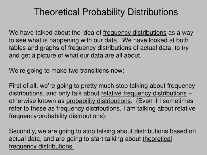
1. Theoretical Probability Distributions We have talked about the idea of frequency distributions as a way to see what is happening with our data. We have looked at both tables and graphs of frequency distributions of actual data, to try and get a picture of what our data are all about. We’re going to make two transitions now: First of all, we’re going to pretty much stop talking about frequency distributions, and only talk about relative frequency distributions – otherwise known as probability distributions. (Even if I sometimes refer to these as frequency distributions, I am talking about relative frequency/probability distributions). Secondly, we are going to stop talking about distributions based on actual data, and are going to start talking about theoretical frequency distributions.

2. Theoretical Probability Distributions A theoretical probability distribution is a distribution that can be described by a mathematical formula. We don’t have actual data with a theoretical distribution, but some theoretical distributions are very useful because lots of real data situations are distributed in ways that are close to those theoretical distributions. This is important because the mathematical formulae let us figure things out about the distribution that we couldn’t easily figure out if we just made distributions based on some data.

3. Let’s look at an example of a very simple theoretical probability distribution: the rectangular distribution. f(x) = c What this formula tells us is that the frequency of our variables is equal to c. What is c? c stands for a constant. What this formula is telling us is that no matter what x is, the relative frequency (the probability) will be the same.

4. f(x) = c Because c in this formula is a constant, but we haven’t said what specific constant it is, this formula doesn’t really tell us about any specific frequency distribution. This formula tells us about a whole family of distributions. For any specific distribution, we have to have a specific value of c. So, if we want to have a specific rectangular distribution, we have to say what c is. So, if we want to have a specific rectangular distribution, we need to say what c is. For example, f(x) = 16.67%

5. f(x) = 16.67% This formula tells us that the probability of any value of x is 16.67% If we graph this distribution, it looks like this:

6. On the other hand, we could have a different rectangular distribution: f(x) = 25%. This tells us that the probability of every value of x is .25 (25%). A graph of this would look like this:

7. You can see why we call this a rectangular distribution. Even though these are two different formulas, they have a ‘family resemblance,’ and the graphs of them will look similar. f(x) = 16.67% f(x) = 25%

8. This discussion has all been pretty abstract. To take a more concrete example – although one made up – imagine that we do a study where we take a random sample of students from a high school. If we ask each person in our sample what grade they are in, we might expect a rectangular distribution: f(x) = 25%

9. The Normal Distribution The rectangular distribution is really only useful in a limited number of situations. A much more important theoretical distribution – although one with a more complex formula – is the normal distribution. The normal distribution is important for two reasons: A lot of variables are distributed like a normal distribution (Height, Weight, IQ). The normal distribution plays an important role in inferential statistics.

10. The Normal Distribution The normal distribution is the familiar bell-curve that you’ve probably all seen. The normal distribution is symmetrical (skew = 0), and the mean, median, and mode are all equal. Median Mode

11. The Normal Distribution Like the rectangular distribution, the normal distribution has a formula. The formula looks like this: f(x) = DON’T WORRY: YOU DON’T HAVE TO UNDERSTAND THIS FORMULA!!!! I mainly just want to make the point that like all theoretical distributions, this one has a formula. Also, like the rectangular distribution, this formula really describes a family of distributions.

12. The Normal Distribution You can see that each of these distributions looks like a bell curve. But, each one has a different mean (µ) and a different variance (σ2). In other words, instead of c (like in the rectangular distribution), the normal distribution has two things we need to know: µ & σ2 (or σ).

13. The Area Under a Curve With a frequency distribution drawn like this, there is a direct connection between the “geometry” of the curve and the numbers that it represents.

14. Imagine that the curve is filled in with circles, each one standing for a person (or other object) represented in the graph. In this example, there are 114 circles, which we can pretend represent 114 people (in real examples, there may be many many more people). For example, suppose we measured the heights of 114 people, and made a frequency polygon. 114 people represents 100% of the heights of people in this distribution. 66in

15. But, what if we wanted to know what percentage of the people in our distribution were 6-feet or taller? We can look at how many circles – how much space or area – is taken up under the graph from 72 inches (6 feet) and higher. In this example, that’s 5 circles. (What percent of 114 is that?) 66 in 72 in

16. For one more example, what if we wanted to know how many people were between 5 and 6 feet tall? We can look at that area under the curve, and figure that out too. Of course, this works out to 104 circles (114 - 5 - 5), or about 91.23% of the area under the curve. 60 in 66in 72 in

17. What if we wanted to know how many people were shorter than 5-feet (60 in)? Again, we can see that the space taken up is filled by 5 circles – about 4.39% of the total area under the graph and about 4.39% of the people in our study. 60 in 66 in

18. To summarize: The total area under a frequency distribution graph represents 100% of the participants in the data set. We can look at the amount of area that is cut off by certain points on the X axis, and that will tell us how many participants fall into the range of the points cut off. In our examples, we looked at the range from the 72 inches to the tallest person; we looked at the range of the shortest person to 60 inches; and we looked at the range of people between 60 inches and 72 inches. All of this works for any frequency distribution. However, it is particularly useful for theoretical distributions like the normal distribution. In fact, it is particularly useful for the normal distribution.

19. The Normal Distribution Because the normal distribution is symmetrical, and because the mean is equal to the median, we know that the area above the mean and the area below the mean is equal to 50% (.5) of the distribution: 0.5 0.5 Median Mode

20. The Normal Distribution The Normal Distribution also allows us to use the “1-2-3 Rule”: If a variable is distributed as a normal distribution, then approximately 68% of the people in the study will have values on the variable between 1 standard deviation below the mean and 1 standard deviation above the mean; approximately 95% of the people will have scores between 2 sd above and below the mean, and approximately 99% of the people will have scores between 3 sd below & above the mean.

21. 57 in 60 in 63 in 66 in 69 in 72 in 75 in The Normal Distribution Think about our height example from before. The mean was μ = 66 inches. Imagine that the standard deviation was σ = 3 in. We would therefore know that about 68% of the people were between 63 and 69 in (66 -3 and 66 + 3). We would know that about 95% of the people were between 60 and 72 in, and we would know that almost all of the people (about 99% were between 57 and 75 in

22. 57 in 60 in 63 in 66 in 69 in 72 in 75 in Using the Normal Distribution So, we have learned that we can figure out what percentage of cases in our data set fall in certain ranges. Approximately 68% fall between 1 sd above and below the mean, approximately 95% fall between 2 sd above and below the mean, and approximately 99% fall between 3 sd above and below the mean. But, what if we want to figure out how many people are in some other range? For example, what if we want to know how many people are taller than 5 ft 7 and 1/4 in (67.25 in)?

23. Using The Normal Distribution How many people are 67.25 inches or taller? μ = 66 in σ = 3 in 67.25 in

24. If we knew calculus, this would be a doable problem. But, since I’m assuming most of you aren’t eager to learn calculus right now, we will learn some other ways to do it. We will learn two methods: One way is to have SPSS calculate the probabilities for you: that is, the computer will do the calculus for us. The other way is to use something called the standard normal distribution and z-scores.