Download
1 / 30
320 likes | 568 Vues
7. Theoretical Probability Distributions. Random variables (RV) Represented by X,Y, or Z Discrete or continuous RV Discrete RV martial status: single, married, divorced Continuous RV weight, height. 7.1 Probability distributions Every RV has a corresponding probability distribution.

E N D
7 Theoretical Probability Distributions
Random variables (RV) Represented by X,Y, or Z Discrete or continuous RV Discrete RV martial status: single, married, divorced Continuous RV weight, height
7.1 Probability distributions Every RV has a corresponding probability distribution. X = the birth order of each child born to a woman residing in US X = 1, 2 first-born, second-born child Let X = the RV, x = the outcome of a particular child P(X=4) = 0.058 P(X=1 or X=2) = 0.416 + 0.330 = 0.746 Chapter7 p163
7.1 Probability distributions Probability distribution of Table 7.1 data. Probabilities that are calculated (from a finite amount of data, based on theoretical consideration) are called (empirical, theoretical) probabilities. Chapter7 p164
7.2 The binomial distribution Dichotomous RV, Y = life and death, male and female, sickness and health Also known as Bernoulli RV Example Y denotes smoking status, Y=0,1 non-smoking, smoking In 1987, 29% of the adults in the US smoked cigar, cigarettes or pipes P(Y=1) = p = 0.29 P(Y=0) = 0.71 X denotes the number of persons selected from the population of adults in the US X can take on three possible values: 0, 1, 2 P(X=0) = (1-p)(1-p) = 0.504 P(X=1) = p(1-p) + (1-p)p = 0.412 P(X=2) = p*p = 0.084 P(X=0) + P(X=1) + P(X=2) = 1
7.2 The binomial distribution X would be a binomial RV with parameters n=3 and p=0.29 P(X=0) = (1-p) (1-p) (1-p) = 0.358 P(X=1) = p(1-p) (1-p) + (1-p)p (1-p) + (1-p) (1-p)p = 0.439 P(X=2) = p*p (1-p) + p (1-p)p + (1-p)p*p = 0.179 P(X=3) = p*p*p = 0.024 In case X=n (mean,variance) of X = (np, np(1-p)) For n=10, (np, np(1-p)) = (10*0.29, 10*0.29*(0.71) = (2.9, 2.059)
Skew to right = = Chapter7 p171
symmetric = = Chapter7 p172
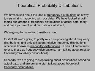
7.3 The Poisson distribution When n>>1, and p is very small, such as p = the probability of a person involved in a motor vehicle accident each year in the US = 0.00024 The Poisson distribution is used to model disctete events that occur infrequently in time or space. X is said to have a Poisson distribution with parameter l
7.3 The Poisson distribution • Binomial distribution, np, np(1-p), if p <<1 • np, np mean = variance Example Determine the number of people in a population of 10000 who will be involved in a motor vehicle accident per year l = 10000*0.00024 = 2.4
= l Chapter7 p175
The Poisson distribution is highly skewed for small l, as l increases, the distribution becomes more symmetric. Chapter7 p175
The Poisson distribution is highly skewed for small l, as l increases, the distribution becomes more symmetric. Chapter7 p175
7.4 The Normal distribution • Discrete binomial or Poisson distribution • as n increases Normal distribution where -∞<x< ∞ = = Chapter7 p177
7.4 The Normal distribution Change of variable standard normal distribution With mean m=0, variance s2= 1 Chapter7 p177
=- = Chapter7 p179
Figure 7.10 The standard normal curve, area between z = -2.00 and z = 2.00 Chapter7 p180
= Chapter7 p181
NORMDIST - Area under the curve start from left hand side Z=0 Z=2
Let X = systolic blood pressure. For the population of 18- to 74-year-old males in the US, systolic 收縮的blood pressure is distributed with a mean 129 mm Hg and standard deviation 19.8 mm Hg. • Find the value of x that cuts off the upper 2.5% of the curve of systolic blood pressure, • Find P(X>x) = 0.025 for the upper 2.5% • z = 1.96 = (x – 129)/ 19.8 • x = 167.8 mm Hg Symmetric (the lower 2.5%) z = -1.96 x = 90.2 mm Hg Chapter7 p182
Comparison of two normal distributions (ND) • Not taking corrective medication, diastolic 舒張 blood pressure is approximately ND with • mean = 80.7 mm Hg, s.d = 9.2 mm Hg • For the men using antihypertensive drugs, with • mean = 94.9 mm Hg, s.d = 11.5 mm Hg • Example • Identify 90% of the persons who are currently taking medication, what value of diastolic blood pressure should be designated as the lower cutoff point ? • From Table, lower 10% z = -1.28 x = 80.2 mm Hg • Below 80.2 mm Hg represent FN • Person who is taking medication are not identified as such
Other probability distributions Negative binomial distribution, multi-nomial distribution, hypergeometric distribution Negative binomial distribution When X=x, among the previous x-1 test, r-1 times are success, x-r times are failure Example A telegraph system has a probability of 0.1sending wrong message. What is the probability that the 10th message is the third error ?
Multi-nomial distribution n independent tests, each test has r types of outcome, where each type has a probability of occurrence p1, ….., pr. Let the RV be X=(X1, ….Xr). Example A dice is thrown 10 times, what is the probabilities that number 1,3 and 5 occur 2,3,and 5 times respectively ?
Hypergeometric distribution N balls, R red color balls, N-R white color balls, RV, X = n balls are drawn without replacement X is said to have hypergeometric distribution - the probability of having x red ball from R red balls, and n-x white ball for N-R white balls. Example A cargo of 50 goods, 5 are defected and 45 are good. Five pieces are drawn, what is the probability of identify defected goods ? P(X≧1) = 1 – P(X≦0) = 1-f(0)
7.5 Further applications Chapter7 p189