Download
1 / 32
330 likes | 1.02k Vues
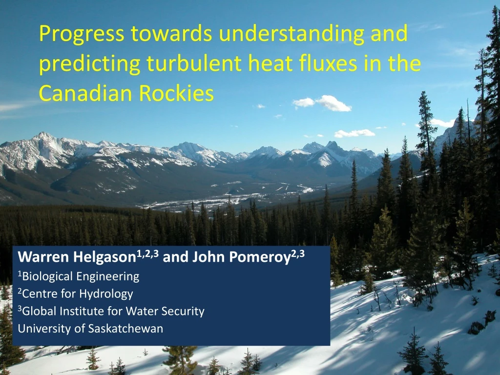
Progress towards understanding and predicting turbulent heat fluxes in the Canadian Rockies. Warren Helgason 1,2,3 and John Pomeroy 2,3 1 Biological Engineering 2 Centre for Hydrology 3 Global Institute for Water Security University of Saskatchewan.

E N D
Progress towards understanding and predicting turbulent heat fluxes in the Canadian Rockies Warren Helgason1,2,3 and John Pomeroy2,3 1Biological Engineering 2Centre for Hydrology 3Global Institute for Water Security University of Saskatchewan
energy to snowpack = net radiation + sensible heat + latent heat radiation exchange (solar + thermal) Q* sensible heat latent heat QH QE = λE snowpack QK heat transfer to snowpack soil Background: Snow energy modeling
convective heat and mass transfer q u T wind temp. vapour snowpack soil Background: Estimating turbulent transfer
Problems with flux estimation approaches? • 1storder flux estimation techniques are commonly employed in land-surface schemes, hydrological models, and snow physics models • Assumptions: • Fluxes are proportional to the vertical gradients of the mean concentration • Production of turbulent energy is approximately equal to dissipation of energy • There have been very few investigations of turbulent structure in mountain environment
Objectives: • Characterize the near-surface structure of the turbulent boundary layer within a mountain valley • Assess the suitability of 1st-order (flux-gradient) estimation techniques Looking forward: Suggest future observational and modelling studies to address key knowledge gaps
Measurement tower Internal Boundary Layer Equilibrium Boundary Layer Methodology: Internal Boundary Layer Equilibrium boundary layer: (turbulence production = dissipation) flow is in 'equilibrium with local surface' Strategy: make measurements in a locally homogeneous area Compare turbulence statistics between measurement sites and with theory
Primary Study Location: Marmot Basin • Hay Meadow: • large, open clearing • local elevation: 1350m • surrounding mountains: 2700m • level topography • fetch: 100-200m Bow River valley Ridge-top stn. Wind direction Hay Meadow Kananaskis River valley
Comparison Locations Wolf Creek, YT subarctic tundra cordillera Saskatoon, SK agricultural prairie Marmot Creek, AB subalpine forest
Alpine site: Wolf Creek, YT Wind direction E.C. sled
Prairie site: Saskatoon, SK snow depth ~ 45 cm
Turbulent Flux Measurement Eddy Covariance Technique • 20 hz. measurements u,v,w,Ts,q • 30 min. covariances sensible heat flux sonic anemometer latent heat flux krypton hygrometer momentum flux friction velocity
Valley sites are typically calm Marmot Valley Spray Valley Prairie Alpine ridge
Log-linear profiles do exist, but... Measured fluxes do not agree with mean gradient predictions
Valley wind speeds are typically low, but often gusty * measured at 2m height NOTE THE AXIS ARE WRONG ON THE FIGURE!!!! * measured at 10m height
Valley sites have the highest intensity of turbulence Marmot Valley Spray Valley Prairie Alpine ridge
Turbulence Characteristics • not all motions contribute to fluxes... • mountain valleys have very low correlation between u, and w • horizontal variance is larger than vertical (due to blocking) Spray Valley Marmot Valley Prairie Alpine ridge typical atmospheric value: -0.35
Spectra –wind velocity components Hay Meadow Both horizontal and vertical spectra exhibit enhanced energy at low frequencies ‘Kansas’
Cospectra – momentum and heat flux co-spectra peak at lower frequencies wind gusts cannot be considered 'inactive' turbulence
Much of the flux contributed by gusts e.g. motions that occupy 10% of the time, account for almost 60% of the flux!
upper level winds strong shear zone detached eddies core valley winds tributary valley winds surface winds (internal B-L) flux tower in clearing Conceptual model drainage winds
Fluxes in mountain valley sites are strongly influenced by non-local processes How does this impede the ability to accurately model the fluxes?
Momentum transfer is significantly enhanced, but still proportional to the wind speed gradient Marmot Valley Prairie Spray Valley Alpine ridge
Heat and mass transfer coefficients are poorly estimated from momentum transfer
Modeling the mountain valley fluxes required environment-specific parameters
Summary of Observations • wind gusts are a source of turbulent energy that don’t scale on local processes. • boundary layer is not in equilibrium • 1st order flux estimation not valid ... but can be made to work with empirical factors These results are not unique to this basin!
Future Directions • Develop flux estimation techniques that incorporate non-local contributions (empirically, statistically, or physically based) • Need to understand turbulent wind structure at multiple scales • regional synoptic forcing • mountain valley climate system • local winds (drainage, land cover) • turbulent scales (emphasis on larger eddies containing the energy)
Combined observation / modelling • surface winds: micrometeorological equipment • vertical structure: SODAR w / windRASS • windflowpatterns: mesoscale model (WRF, meso-NH, etc.) • fine scale turbulence: large eddy simulation nested (2-way) within mesoscale model
Future Plans: • Fall 2013 - resume turbulence observations; mesoscale weather model setup • Summer 2014 - intensive field campaign • Fall 2014 - detailed modelling (Nested LES)