Download
1 / 16
220 likes | 435 Vues
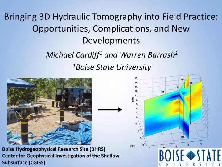
Bringing 3D Hydraulic Tomography into Field Practice: Opportunities, Complications, and New Developments. Michael Cardiff 1 and Warren Barrash 1 1 Boise State University. Boise Hydrogeophysical Research Site (BHRS) Center for Geophysical Investigation of the Shallow Subsurface (CGISS).

E N D
Bringing 3D Hydraulic Tomography into Field Practice:Opportunities, Complications, and New Developments Michael Cardiff1 and Warren Barrash1 1Boise State University Boise Hydrogeophysical Research Site (BHRS) Center for Geophysical Investigation of the Shallow Subsurface (CGISS)
Detailed Hydraulic Conductivity Data:A Continuing Challenge • Where will contaminants go? • How much mixing will take place? • Where are aquifers highly “connected”? Current options: • Partially-penetrating slug tests • Borehole flowmeters • Borehole geophysical methods • Geophysical tomography methods 1D, 2D, or 3D Variability 1D (Vertical Variability)
3D Hydraulic Tomography (HT):A “New” Characterization Approach • Data Collection Phase • Perform pumping from a discrete interval • Measure head changes at many discrete intervals in several wells • Repeat for several arrangements • Analysis Phase • Image subsurface hyd. conductivity (K) through inversion • Benefits: • Directly sensitive to K • Provides information about connectivity of high-K zones • Does not make homogeneity or “effective” parameter assumptions • Drawbacks: • Requires a detailed numerical model and moderate to high computational power • Equipment-intensive and possibly time-intensive • Imaging accuracy decreases with increasing distance from pumping and observation locations
Open Questions • Can HT be made practical for field characterization? • Equipment challenges • Computational challenges • What “nuisance effects” impact quality of HT data and analysis? • E.g. borehole deviation, wellbore skin, wellbore hydraulics
Testing HT at Boise Hydrogeophysical Research Site (BHRS) • Permeable, unconsolidated and unconfined sand and gravel aquifer • Weakly heterogeneous (1-2 order of mag. K variation) • 15m thick • 18 fully-penetrating wells • Other hydrologic datasets (2,500 slug test records) available
Field Campaign – Aug 1-6, 2010 • Pumped at successive 1m intervals in B4 and B5 (12 tests per well) • 7 observation intervals (every 2m) in wells B1, B2, C3, C4
HT Implementation Hardware: • Custom multi-level packer/port systems • Fiberoptic pressure transducers • Custom-designed Labview data acquisition software (50 simultaneous data streams) Analysis Software: • MATLAB inversion software • MODFLOW model with ADJ (adjoint) sensitivity analysis process Visualization from HT software showing pumping problems A fiberoptic pressure transducer, with marker for scale HT setup showing pumping and monitoring wells (foreground) HT pumping and monitoring run from back of a van
HT Data HT Head Change (drawdown) curves for one pumping test, one observation well
HT Inversion Results • ≈300 datapoints fit (3 per drawdown curve) • Data inverted using geostatistical inversion (Kitanidis, 1995) • Regularization tied to geostatistics • Produces uncertainty metrics in addition to image • ≈80K parameters estimated (K in 1m x 1m x 0.6m blocks) Inversion results (K in m/s) along slices through observation wells
HT Inversion Results – Data Fit Histogram of residuals for all data. Standard deviation = 2.0mm Histogram of residuals for inverted data. Standard devation = 2.1mm Cross-plot between inverted field data and simulated observations
HT Inversion Results – Validation Comparison between HT and slug test data: • Similar trends in relative magnitude • Fine-scale variability not recovered • K values from HT are lower, more consistent with other historical tests (e.g. fully-penetrating pumping) Slug test data in: Cardiff, Barrash, Malama & Thoma (2011) JoH
Effects of non-ideal conditions? Modeling: • Usually, assume pumping is a “point” source with known location The Real World: • Complex well hydraulics • Wellbore skin effects • Wellbore deviation Difficulties encountered in real-world applications
Comparing FE models with detailed wellbore geometry HT data relatively insensitive to: • Near-wellbore skin • Existence of in-well impermeabilities (packers) and open intervals (ports) …but, sensitive to moderate wellbore deviation!
Ongoing work Pumping Strategy • Refinement of HT components for increased flexibility and automation • Testing of alternative stimulation (pumping) strategies • Implementation at a “real” site! Interested? Pressure Transducers Packer / Port Hardware Data Acquisition System Numerical Model Inversion Code
Conclusions • Hydraulic tomography can estimate feature connectivity patterns that may be difficult to detect with other methods • Careful design of data collection strategies, accurate data, and good numerical modeling are all key • Treating pumping and observation intervals as points is an adequate strategy for modeling • A portable installation for HT investigations is being refined for future field applications
Thank you!Questions? Contact: Michael Cardiff MichaelCardiff@boisestate.edu (208)-426-4678 HT Funding Support: Primary support from NSF-CMG (Collaboration in Mathematics and Geosciences, DMS-0934680) Additional support from: NSF Grant EAR-0710949 EPA Grants X-96004601-0 and -1 US Army RDECOM ARL ARO grant W911NF-09-1-0534 Slug testing support: NSF grant EAR-0710949 EPA grants X-96004601-0 and -1