Download
1 / 36
360 likes | 369 Vues
Histograms. CSE 4309 – Machine Learning Vassilis Athitsos Computer Science and Engineering Department University of Texas at Arlington. Input Image. Example Application: Skin Detection. Goal: find skin pixels in the image. In the output: White pixels are pixels classified as “skin”.

E N D
Histograms CSE 4309 – Machine Learning VassilisAthitsos Computer Science and Engineering Department University of Texas at Arlington
Input Image Example Application: Skin Detection • Goal: find skin pixels in the image. • In the output: • White pixels are pixels classified as “skin”. • Black pixels are pixels classified as “not skin”. • This is an opportunity to talk about images. • We will use images as data in several cases this semester. Example Output Image
Input Image Pixel-Based Skin Detection • In pixel-based skin detection, each pixel is classified as skin or non-skin, based on its color. • No other information is used. • Each pixel is classified independently of any other pixel. • So, the input space is the space of 3D vectors (r, g, b), such that r, g, b are integers between 0 and 255. • The output space is binary ("skin" or "non skin"). Output Image
Example Application: Skin Detection • Why would skin detection be useful?
Example Application: Skin Detection • Why would skin detection be useful? • It is very useful for detecting hands and faces. • It is used a lot in computer vision systems for person detection, gesture recognition, and human motion analysis.
Examples of Skin Detection Output Image Input Image • The classifier is applied individually on each pixel of the input image. • In the output: • White pixels are pixels classified as “skin”. • Black pixels are pixels classified as “not skin”.
Examples of Skin Detection Output Image Input Image • The classifier is applied individually on each pixel of the input image. • In the output: • White pixels are pixels classified as “skin”. • Black pixels are pixels classified as “not skin”.
Building a Skin Detector • We want to classify each pixel of an image, as skin or non-skin. • What is the input to the classifier?
Building a Skin Detector • We want to classify each pixel of an image, as skin or non-skin. • What is the input to the classifier? • Three integers: R, G, B. Each is between 0 and 255. • The red, green, and blue values of the color of the pixel. • If we want to use a Bayes classifier, which probability distributions do we need to estimate?
Estimating Probabilities • If we want to use a pseudo-Bayes classifier, which probability distributions do we need to estimate? • p(skin | R, G, B) • p(not skin | R, G, B) • To compute the above probability distributions , we first need to compute: • p(R, G, B| skin) • p(R, G, B| not skin) • p(skin) • p(not skin)
Estimating Probabilities • We need to compute: • p(R, G, B | skin) • p(R, G, B | not skin) • p(skin) • p(not skin) • To compute these quantities, we need training data. • We need lots of pixels, for which we know both the color and whether they were skin or non-skin. • p(skin) is a single number. • How can we compute it?
Estimating Probabilities • We need to compute: • p(R, G, B | skin) • p(R, G, B | not skin) • p(skin) • p(not skin) • To compute these quantities, we need training data. • We need lots of pixels, for which we know both the color and whether they were skin or non-skin. • p(skin) is a single number. • We can simply set it equal to the percentage of skin pixels in our training data. • p(not skin) is just 1 - p(skin).
Estimating Probabilities • How about p(R, G, B| skin) and p(R, G, B| not skin)? • How many numbers do we need to compute for them?
Estimating Probabilities • How about p(R, G, B| skin) and p(R, G, B| not skin)? • How many numbers do we need to compute for them? • How many possible combinations of values do we have for R, G, B?
Estimating Probabilities • How about p(R, G, B| skin) and p(R, G, B| not skin)? • How many numbers do we need to compute for them? • How many possible combinations of values do we have for R, G, B? • 2563= 16,777,216 combinations. • So, we need to estimate about 17 million probability values for p(R, G, B| skin) • Plus, we need an additional 17 million values for p(R, G, B | not skin)
Estimating Probabilities • So, in total we need to estimate about 34 million numbers. • How do we estimate each of them? • For example, how do we estimate p(152, 24, 210 | skin)?
Estimating Probabilities • So, in total we need to estimate about 34 million numbers. • How do we estimate each of them? • For example, how do we estimate p(152, 24, 210 | skin)? • We need to go through our training data. • Count the number of all skin pixels whose color is (152,24,210). • Divide that number by the total number of skin pixelsin our training data. • The result is p(152, 24, 210 | skin).
Estimating Probabilities • How much training data do we need?
Estimating Probabilities • How much training data do we need? • Lots, in order to have an accurate estimate for each color value. • Even though estimating 34 million values is not an utterly hopeless task, it still requires a lot of effort in collecting data. • Someone would need to label billions of pixels as skin or non skin. • While doable (at least by a big company), it would be a very time-consuming and expensive undertaking.
Histograms • Our problem is caused by the fact that we have to many possible RGB values. • Do we need to handle that many values?
Histograms • Our problem is caused by the fact that we have to many possible RGB values. • Do we need to handle that many values? • Is p(152, 24, 210 | skin) going to be drastically different than p(153, 24, 210 | skin)? • The difference in the two colors is barely noticeable to a human. • We can group similar colors together. • A histogram is an array (one-dimensional or multi-dimensional), where, at each position, we store the frequency of occurrence of a certain range of values. Color: (152, 24, 210) Color: (153, 24, 210)
Histograms • For example, if we computed p(R, G, B | skin) for every combination, the result would be a histogram. • More specifically, it would be a three-dimensional 256x256x256 histogram (a 3D array of size 256x256x256). • Histogram[R][G][B] = frequency of occurrence of that color in skin pixels. • However, a histogram allows us to group similar values together. • For example, we can represent the p(R, G, B| skin) distribution as a 32x32x32 histogram. • To find the histogram position corresponding to an R, G, B combination, just divide R, G, Bby 8, and take the floor.
Histograms • Suppose that we represent p(R, G, B | skin) as a 32x32x32 histogram. • Thus, the histogram is a 3D array of size 32x32x32. • To find the histogram position corresponding to an R, G, B combination, just divide R, G, B by 8, and take the floor. • Then, what histogram position corresponds to RGB value (152, 24, 210)?
Histograms • Suppose that we represent p(R, G, B | skin) as a 32x32x32 histogram. • Thus, the histogram is a 3D array of size 32x32x32. • To find the histogram position corresponding to an R, G, B combination, just divide R, G, B by 8, and take the floor. • Then, what histogram position corresponds to RGB value (152, 24, 210)? • floor(152/8, 24/8, 210/8) = (19, 3, 26). • So, to look up the histogram value for RGB color (152, 24, 210), we look at position [19][3][26] of the histogram 3D array. • In this case, each position in the histogram corresponds to 8x8x8 = 512 distinct RGB combinations. • Each position in the histogram is called a bin, because it counts the frequency of multiple values.
How Many Bins? • How do we decide the size of the histogram? • Why 32x32x32? • Why not 16x16x16, or 8x8x8, or 64x64x64?
How Many Bins? • How do we decide the size of the histogram? • Why 32x32x32? • Why not 16x16x16, or 8x8x8, or 64x64x64? • Overall, we have a tradeoff: • Larger histograms require more training data. • If we do have sufficient training data, larger histograms give us more information compared to smaller histograms. • If we have insufficient training data, then larger histograms give us less reliable information than smaller histograms. • How can we choose the size of a histogram in practice?
How Many Bins? • How do we decide the size of the histogram? • Why 32x32x32? • Why not 16x16x16, or 8x8x8, or 64x64x64? • Overall, we have a tradeoff: • Larger histograms require more training data. • If we do have sufficient training data, larger histograms give us more information compared to smaller histograms. • If we have insufficient training data, then larger histograms give us less reliable information than smaller histograms. • How can we choose the size of a histogram in practice? • Just try different sizes, see which one is the most accurate.
The Statlog Dataset • Another dataset that we will use several times in this course, is the UCI Statlog dataset(we also call it the Satellite dataset). • Input: a 36-dimensional vector, describing a pixel in an image taken by a satellite. • The value in each dimension is an integer between 1 and 157. • Why 36 dimensions? • To describe each pixel, four basic colors are used, instead of the standard three colors (r, g, b) we are used to. • To classify a pixel, information is used from its 8 neighboring pixels. So, overall, 9 pixels x 4 colors = 36 values. • Output: type of soil shown on the picture. 1: red soil 2: cotton crop 3: grey soil 4: damp grey soil 5: soil with vegetation stubble 7: very damp grey soil
Limitations of Histograms • For skin detection, histograms are a reasonable choice. • How about the satellite image dataset? • There, each pattern has 36 dimensions (i.e., 36 attributes). • What histogram size would make sense here?
Limitations of Histograms • For skin detection, histograms are a reasonable choice. • How about the satellite image dataset? • There, each pattern has 36 dimensions (i.e., 36 attributes). • What histogram size would make sense here? • Even if we discretize each attribute to just two values, we still need to compute 236values, which is about 69 billion values. • We have 4,435 training examples, so clearly we do not have enough data to estimate that many values.
Naïve Bayes with Histograms • The naive Bayes classifier assumes that the different dimensions of an input vector are independent of each other given the class. • Using the naïve Bayes approach, what histograms do we compute for the satellite image data?
Naïve Bayes with Histograms • The naive Bayes classifier assumes that the different dimensions of an input vector are independent of each other given the class. • Using the naïve Bayes approach, what histograms do we compute for the satellite image data? • Instead of needing to compute a 36-dimensional histogram, we can compute 36 one-dimensional histograms. • Why?
Naïve Bayes with Histograms • The naive Bayes classifier assumes that the different dimensions of an input vector are independent of each other given the class. • Using the naïve Bayes approach, what histograms do we compute for the satellite image data? • Instead of needing to compute a 36-dimensional histogram, we can compute 36 one-dimensional histograms. • Why? Because of independence. We can compute the probability distribution separately for each dimension. • p(X1, X2, …, X36 | Ck) = ???
Naïve Bayes with Histograms • The naive Bayes classifier assumes that the different dimensions of an input vector are independent of each other given the class. • Using the naïve Bayes approach, what histograms do we compute for the satellite image data? • Instead of needing to compute a 36-dimensional histogram, we can compute 36 one-dimensional histograms. • Why? Because of independence. We can compute the probability distribution separately for each dimension. • p(X1, X2, …, X36 | Ck) = p1(X1| Ck) * p2(X2| Ck) * … * p36(X36| Ck)
Naïve Bayes with Histograms • Suppose that build these 36 one-dimensional histograms. • Suppose that we treat each value (from 1 to 157) separately, so each histogram has 157 bins. • How many numbers do we need to compute in order to compute our p(X1, X2, …, X36 | Ck) distribution?
Naïve Bayes with Histograms • Suppose that build these 36 one-dimensional histograms. • Suppose that we treat each value (from 1 to 157) separately, so each histogram has 157 bins. • How many numbers do we need to compute in order to compute our p(X1, X2, …, X36 | Ck) distribution? • We need 36 histograms (one for each dimension). • 36*157 = 5,652 values. • Much better than 69 billion values for 236 bins. • We compute p(X1, X2, …, X36 | Ck) for six different classes c, so overall we compute 36*157*6 = 33,912 values.