Download

1 / 23
230 likes | 463 Vues
Crosstabs. When to Use Crosstabs as a Bivariate Data Analysis Technique. For examining the relationship of two CATEGORIC variables For example, do men and women (variable is GENDER) have different distributions for the variable SUPER BOWL WATCHING — often, sometimes, never?

E N D
When to Use Crosstabs as a Bivariate Data Analysis Technique For examining the relationship of two CATEGORIC variables • For example, do men and women (variable is GENDER) have different distributions for the variable SUPER BOWL WATCHING — often, sometimes, never? • Ask class for more examples! Both variables must be categoric — nominal, ordinal, or dichotomous.
What is a Crosstab? A cross-tab is a table that displays a joint distribution — a distribution of cases for two variables. It is also called a “contingency table.” Each cell displays the observed count of the cases that fall into a specific category of the IV AND a specific category of the DV.
How to Set Up a Crosstab Decide which variable is the IV and which is the DV. (If you can’t decide, make two tables, one for each option.) Place the IV in the columns. Each COLUMN represents a CATEGORY OF THE IV. The DV goes in the rows. Each ROW represents a CATEGORY OF THE DV.
Cells and Marginals [1] After the observed counts are placed in the cells, a new final column is created at the far right side of the table to display the row totals (or “row marginals”), adding the cell counts ACROSS. And a new row is created at the bottom of the table to display the column totals (or “column marginals”), adding the counts down the columns.
Example: Super Bowl Watching by Gender SUPER BOWL WATCHING BY GENDER
Crosstabs Features Here the IV (gender) is in the columns — two columns are for the two categories of the variable (men and women) and the last column shows the total in each row. Three rows are for the three “Super Bowl watching” categories: often, sometimes, and never. The bottom row shows the totals in each column. The number at the far lower right of the table shows the total number of cases.
Cells and Marginals [2] The marginals — the row and column totals —are “fixed” — they must correspond to the frequency distributions of the variables that exist regardless of the relationship. The row totals are the frequency distribution of the DV. The column totals are the frequency distribution of the IV. More than one distribution is possible for the cell frequencies. Do they show a relationship?
Next? • The next step is to compute percentages for the table, computing within categories of the IV (i.e., in the direction of the IV — GENDER, in this case). • What % of men watch often? What % of men watch sometimes? What % of men watch never? And then what are the corresponding percentages for women? • Each column’s percentages must add up to 100%. • Are these two % distributions (one for men and one for women) similar to each other or not?
ONLY COMPUTE PERCENTAGES DOWN THE COLUMNS! We could percentage the table across rows, down columns, or with each cell count as a proportion of the total — or all of these displayed in the same table. RESIST THE TEMPTATION TO PERCENTAGE EVERYTHING! COMPUTE PERCENTAGES ONLY DOWN THE COLUMNS, IN THE DIRECTION OF THE IV.
WHY? If percentages are computed down the columns, we can see at a glance if the IV categories have similar DV distributions. If we do it any other way, the percentages will be confusing and hard to read.
What Do We Do Now? Look carefully at the DV percentage distributions — do they look similar for the categories of the IV? Compute chi-square to see if the differences are significant. Compute measures of association to see if the relationship is strong.
Significance The chi-square test of significance helps to confirm what we should be able to see by looking at the percentages: Do the IV categories have different proportional (%) distributions into the DV categories? The null hypothesis is that their DV distributions are all the same.
Significance of the Relationship The test of significance for a crosstab is called chi-square. (That’s a “K” sound in chi!) The chi-square test statistic measures the discrepancy between the observed distribution and a hypothetical “null hypothesis” distribution. The null hypothesis is that all categories of the IV have an identical distribution into the DV categories. (Men and women have identical distributions into the super bowl watching categories.)
How to Calculate Chi-SquareStep 1: The Expected Counts [1] Compute expected counts for each cell, under the hypothesis of identical proportional DV distributions for all IV categories. In each cell, the expected count is calculated as the row total for the row the cell is in multiplied by the column total for the column the cell is in, and divided by the total sample size. E = (row total)(column total) / N
Expected Counts [2] E = CR/N The logic is that the row total divided by the grand total (sample size) represents the proportion of cases in the column that we would expect to find in this particular cell if there were no differences among the IV categories in their DV distributions (if men and women watched the Super Bowl in the same proportions). To get the expected count of cases in the cell, we apply that proportion — row total / N — to the column total by multiplying: (column total)(row total) / N = expected count in the cell
Now Compute Chi-Square After we have computed all of the expected counts, we compute the overall discrepancy between these expected counts and the observed counts we found in our data. That is the value of chi-square: χ2 = ∑ [(O – E)2 / E] In each cell, we subtract the expected count from the observed count and square the difference. We divide by the expected count for the cell. Then we repeat this calculation for all the cells of the table and sum the results.
Chi-Square and Degrees of Freedom If there are big discrepancies between the expected (null hypothesis) counts and the observed counts, chi-square will be relatively large. We have to calculate the degrees of freedom for our chi-square: df = (r – 1)(c – 1) where r is the number of row (DV) categories and c is the number of column (IV) categories.
OK, Look It Up! Once the df is calculated, we can look up our computed chi-square in the table of its distribution and see if it exceeds the critical value for the degrees of freedom. If it does, we can say that we have found a statistically significant difference among the IV categories for their DV distributions (“men and women report significantly different levels of Super Bowl watching”).
Monkey Business with Chi-Square The chi-square test statistic is very sensitive to sample size. A large sample is quite likely to produce a significant chi-square result even when the differences in the distributions are pretty small.
Measures of Association A “measure of association” is a measure of the strength of the relationship between the variables in the crosstab. Some of them are more appropriate for ordinal data, some for nominal data. They have different ranges and require care in interpretation. Check the “How To” section of the text for more details.
Elaboration: The Third Variable Researchers often introduce a third variable into their crosstab analysis. Like the variables in the original bivariate analysis, the third variable in a crosstab needs to be categoric. It should not have too many categories (two or three)! It is introduced as a “layer variable,” and software will produce a separate crosstab and test of significance of the initial bivariate analysis FOR EACH CATEGORY OF THE LAYER VARIABLE.
Third Variable Example For example, in our GENDER/SUPER BOWL example, we could introduce a variable called AGE as the third variable in an elaboration. It could be coded as “young” or “old” for its two categories. We might find that the initial GENDER/SUPER BOWL relationship is different for older people and younger people. For example, among younger people, there might be very little difference between men and women in their Super Bowl watching, while there is a gender difference in viewing habits among the older respondents.