Download
1 / 40
410 likes | 534 Vues
window. power. power. [10 ,14:30]. X. X. X. X. Visual servo (.2, -.15). Dig(5). Drive (-1). NIR. data. Workspace pan. Lo res. Rock finder. Hi res. Carbonate. [10 ,14:30].

E N D
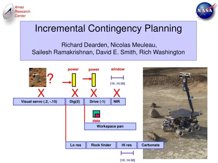
window power power [10 ,14:30] X X X X Visual servo (.2, -.15) Dig(5) Drive (-1) NIR data Workspace pan Lo res Rock finder Hi res Carbonate [10 ,14:30] Incremental Contingency Planning Richard Dearden, Nicolas Meuleau, Sailesh Ramakrishnan, David E. Smith, Rich Washington ?
Why Contingency Planning ?? Limited onboard processing CPU, memory, time Safety sequence checking Anticipation setup steps
The Planning Problem • Given: • start time • pose • energy available • actions with uncertain: • durations • resource usage • Possible science objectives • images • samples Compress ……… Visual servo (.2, -.15) Dig(5) Drive(-1) NIR Drive(2) Warmup NIR Maximize (Expected) Scientific Return
Power Storage Time Visual servo (.2, -.15) Lo res Rock finder NIR Warmup NIR t [10:00, 14:00] E > 2 Ah NIR ∆t = ∆p = Technical Challenges Continuous time (& resources) Continuous outcomes Time (& resource) constraints Concurrency Goal selection & optimization g1, g2, g3, g4 …
Just in Case (JIC) Scheduling 1. Seed schedule 2. Identify most likely failure 3. Generate a contingency branch 4. Integrate the branch .4 .2 .1 • Advantages: • Tractability • Simple plans • Anytime
Just in Case (JIC) Planning 1. Seed plan 2. Identify most likely failure 3. Generate a contingency branch 4. Integrate the branch .4 .2 .1
Expected Utility 20 13:20 15 13:40 10 14:00 5 Power 14:20 Start time 14:40 Limits of JIC Scheduling Heuristics t [9:00, 14:30] = 5s = 1s :most probable failures $ : most interesting branch point • Most probable failure points may not be the best branch-points: • It is often too late to attempt other goals when the plan is about to fail. V = 10 HiRes t [10:00, 14:00] = 600s = 60s = 300s = 5s = 120s = 60s = 1000s = 500s $ V = 100 Visual servo (.2, -.15) Dig(60) Drive (-2) NIR t [9:00, 16:00] = 5s = 1s t [10:00, 13:50] = 600s = 60s = 120s = 20s V = 50 Lo res Rock finder LIB V = 5 Warmup LIB True for all initial states in the grey box. = 1200s = 20s
Just in Case (JIC) Planning ? ? ? ? 1. Seed plan 2. Identify best branch point 3. Generate a contingency branch 5. Evaluate & Integrate the branch Construct plangraph Back-propagate value tables Compute gain Select branch condition & goals Vm Vb r
Construct Plangraph g1 g2 g3 g4
Value Tables V1 g1 r V2 g2 r V3 g3 r V4 g4 r
5 e 1 e Example q g A B (10, 15) (10, 15) p r C (3, 3) g’ E (2, 2) s t D (1, 5)
5 5 e 15 1 e Simple Propagation q g A B (10, 15) (10, 15) p r C (3, 3) g’ E (2, 2) s t D (1, 5)
5 5 5 e 25 15 1 e Simple Propagation q g A B (10, 15) (10, 15) p r C (3, 3) g’ E (2, 2) s t D (1, 5)
5 5 5 e 25 15 1 1 e 2 Simple Propagation q g A B (10, 15) (10, 15) p r C (3, 3) g’ E (2, 2) s t D (1, 5)
5 5 5 e 25 15 1 1 e r 2 1 2 Conjunctions q g A B (10, 15) (10, 15) p t 1 r C 2 (3, 3) g’ E (2, 2) s t D (1, 5)
5 5 5 e 25 15 1 1 e r r 2 1 1 2 5 Propagation q g A B (10, 15) (10, 15) p t 1 r C 2 (3, 3) g’ E (2, 2) s t D (1, 5)
5 5 5 t e 25 1 15 15 t 1 2 t 1 5 1 1 e r r 2 1 1 2 5 Propagation q g A B (10, 15) (10, 15) p r C (3, 3) g’ E (2, 2) s t D (1, 5)
5 5 5 t e 25 1 15 15 t 1 2 t t 1 1 5 5 1 1 e r r 2 1 1 2 5 Combining Tables q g A B (10, 15) (10, 15) p r C (3, 3) g’ E (2, 2) s t D (1, 5)
5 5 5 t e 25 1 15 15 t t 1 1 1 1 5 5 5 5 1 e t r r 1 1 1 2 2 5 Discharging Assumptions q g A B (10, 15) (10, 15) p r C (3, 3) g’ E (2, 2) s t D (1, 5)
5 5 5 e 25 15 1 1 5 5 1 e 1 6 Propagation q g A B (10, 15) (10, 15) p r C (3, 3) g’ E (2, 2) s t D (1, 5)
5 5 5 e 15 25 15 1 1 5 8 1 e 1 6 Combining Tables q g A B (10, 15) (10, 15) p 1 r C 5 (3, 3) g’ E (2, 2) s t D (1, 5)
5 5 5 e 15 25 15 1 1 5 8 1 e 1 6 Combining Tables q g A B 5 (10, 15) (10, 15) p 8 25 1 r C 5 (3, 3) g’ E (2, 2) s t D (1, 5)
5 5 5 e 15 25 15 1 1 5 8 1 e 1 6 Ordering q g A B AB 5 CDE (10, 15) (10, 15) p 8 25 1 r C 5 (3, 3) g’ E (2, 2) s t D DCE (1, 5)
5 5 e 15 1 1 5 8 1 e 1 6 Achieving Multiple Goals g+g’ + g 5 g’ 15 25 30 q g A B 5 (10, 15) (10, 15) p 8 25 1 r C 5 (3, 3) g’ E (2, 2) s t D (1, 5)
g+g’ g 5 5 5 g’ e 15 25 30 15 g+g’ g 5 g’ 8 25 30 1 1 5 8 1 e 1 6 Achieving Multiple Goals q g A B (10, 15) (10, 15) p 1 r C 5 (3, 3) g’ E (2, 2) s t D (1, 5)
g+g’ g 5 5 5 g’ e 15 25 30 15 g+g’ g 5 g’ 8 25 30 1 1 5 8 1 e 1 6 Goal Annotation g g q g A B (10, 15) (10, 15) p g’ 1 r C 5 g’ (3, 3) g’ E (2, 2) s t D g’ g’ (1, 5) g’
Just in Case (JIC) Planning ? ? ? ? 1. Seed plan 2. Identify best branch point 3. Generate a contingency branch 5. Evaluate & Integrate the branch Construct plangraph Back-propagate value tables Compute gain Select branch condition & goals Vm Vb r
V r Estimating Branch Value V1 V r Max V2 V r V3 V r V4
Vb r Plan Statistics resource probability plan value function P Vm r r V1 V2 V3 V4
Vm ∞ Vb Gain = ∫ P(r) max{0,Vb(r) - Vm(r)} dr r 0 Vb r Expected Branch Gain P r V1 V2 V3 V4
Vm Vb r Vb r Selecting the Branch Condition branch condition branch condition P r V1 V2 V3 V4
Vm Vb r Vb r Selecting Branch Goals branch goals g1 P g3 r r V1 g1 V2 g3 V3 V4
Vm Vb r Evaluating the Branch ? ? ? ? 1. Seed plan 2. Identify best branch point 3. Generate a contingency branch 4. Evaluate & integrate the branch Compute value function Compute actual gain
∞ Gain = ∫ P(r) max{0,Vb(r) - Vm(r)} dr 0 Vb r Actual Branch Gain P actual branch condition Vm Vb r r Branch value function
Remarks: Single Plangraph ? ? ? ? 1. Seed plan 2. Identify best branch point 3. Generate a contingency branch 5. Evaluate & Integrate the branch Construct plangraph Back-propagate value tables Compute gain Select branch condition & goals Vm Vb r
Plan Graph V1 g1 r V2 g2 r V3 g3 r V4 g4 r
V1 g1 r V2 g2 r V3 g3 r V4 g4 r Branch Initial Conditions {p} v r {q,r} v r v r {p,r} v v r r
Vm Vb r Single Plangraph Construct single plangraph Back-propagate value tables 1. Seed plan 2. Identify best branch point 3. Generate a contingency branch 4. Evaluate & integrate the branch ? ? ? ? Discharge conditions Compute gain Select branch condition & goals
Visual servo (.2, -.15) Dig(5) Drive (-1) Hi res [11 ,14:00] Lo res Rock finder NIR Warm NIR V = 100 Visual servo Hi res Visual servo NIR V’ = 30 Visual servo (.2, -.15) ? Dig(5) Drive (-1) Hi res Lo res Rock finder NIR Issues Sensor costs Setup steps Utility updates Floating contingencies