Download
1 / 43
490 likes | 767 Vues
CCIR 322-2 Atmospheric Noise. Why do this?. Understand the evolution atmospheric noise measurements Determine what are appropriate values to use from the CCIR documentation Compare CCIR data alternative noise data Define the noise environment so mitigation techniques may be explored.

E N D
Why do this? • Understand the evolution atmospheric noise measurements • Determine what are appropriate values to use from the CCIR documentation • Compare CCIR data alternative noise data • Define the noise environment so mitigation techniques may be explored
What is CCIR 322-2? • Reported background atmospheric noise levels • Evolved into ITU P372-7 • Included man-made and galactic noise • Removed technical background • Used the ARN-2 Radio Noise Recorder • 16 Stations around the globe • Average noise power at each of eight frequencies for fifteen minutes each hour • 13 kHz, 11kHz, 250kHz, 500kHz, 2.5MHz, 5MHz, 10MHz, and 20MHz • 1957-1961 (4 years) → 8640 15-minute measurements → 99.98% • Tracked filtered noise envelope not instantaneous noise • Took high speed data to obtain APDs
What is CCIR 322-2? (cont) • Sectioned the year into seasons and time blocks • Four 90-day seasons • Six 4-hour time blocks • Tracked external antenna noise factor, Fa • Power received through a loss-free antenna Fa = 10*log10(Pn/KToB) • Lists the median value hourly value for each time block, Fam, at 1 MHz • Lists the upper decile (90%) level Du • Calculate noise E-field from Fa, BW, frequency • Use normal or log-normal statistics and graphs to adjust values
Computing CCIR Data +14 dB +16 dB <Emedian> = 50 dB uV/m <E95%> = 64 dB uV/m E95% |99%= 80 dB uV/m
Adjustment to Enoise at 95% Time Availability for Service Probability
RMS Envelope vs Inst. Envelope • Failure mode of receiver sometimes dictates using Inst. Envelope values over RMS Envelope values (eg FSK). • Needed a way to measure the “impulsiveness” of the noise. • Came up with using Vd • Vd = 20 * log10( Arms / Aavg) • Vd for Rayleigh (Gaussian > 0) is 1.05 • Larger Vd mean the more impulsive or less Gaussian the noise
CCIR APD Experimental Setup Instantaneous Noise, Vn • Thanks to Bob Matherson and CCIR IF Inst. Noise Voltage, VIF Atm Noise Instantaneous Noise Envelope, A RMS Noise Envelope, Arms Average Noise Envelope, Aavg
Envelope RMS Voltage (Arms) & Instantaneous Envelope Voltage (A) • Arms is 3dB above rms instantaneous noise voltage VIFrms • APD • Amplitude Probability Distribution or A Posteriori Distribution • Exceedance probability P[A > Arms + D=A0] • Parameterized by Vd - Voltage deviation • Plotted on Rayleigh Probability Paper 0 Rayleigh Vd = 1.05 More Impulsive
CCIR FSK Example Results Time availability as a function of service probability Geneva, Switzerland Summer season: 2000-2400 h Frequency: 50 kHz Bandwidth: 100 Hz Binary errors: 0.05% Montgomery [1954] Model
CCIR Limitation (1983 §1) • "The estimates for atmospheric noise levels given in the Report are for the average background noise level due to lightning in the absence of other signals, whether intentionally or unintentionally radiated. In addition, the noise due to local thunderstorms has not been included. In some areas of the world, the noise from local thunderstorms can be important for a significant percentage of the time."
CCIR Limitations (cont) • “Atmospheric radio noise is characterized by large, rapid fluctuations, but if the noise power is averaged over a period of several minutes, the average values are found to be nearly constant during a given hour variations rarely exceeding ±2dB except near sunrise or sunset, or when there are local thunderstorms.”
CCIR Questions • What should we specify as a service probability 95%? • What is an appropriate level of availability? • How do the values change when we are near lightning?
Electric/Magnetic Field Data (cont) dB(V/m/Hz) Preta 1984
Comparing E-fields and Distance • Lightning E-field data varies with 1/D • E2-E1 = 20*log10(D1/D2) = 20*log10(50km/D2) • For 100 kHz, an Enoise of 80 dB uV/m is equivalent to being 8.7 km from continuous repetitive lightning return strokes! • Can do this for all levels of % Time availability for any Service Probability
Conclusion from CCIR Data • Calculate Noise Level • Specify % Time and Confidence • Alternatively, as a distance to a lightning return stroke. I.e. define this as a ATC constraint
Summary • Reviewed CCIR-322 and current lightning research and found good correlation between both data sets. • Need to set both a not-to-exceed level and a confidence to make a reasonable estimate of noise level or can define a distance to a lightning return stroke. e.g. define this as a ATC constraint. • Need to use nonlinear processing to increase SNR. • Have pieces for a time-domain model.
Mitigation Techniques • Clipping or Blanking based on Vd • Spaulding/Middleton • Modestino/Enge • Using the Loran antenna as a lightning detector/locator • Low frequency signals propagate faster than higher frequency signals • Magnetic antenna / magnetometer
Spaulding/Middleton (Parametric) • Divide all noise into three canonical forms • Class A (3 parameters) • (duration of noise)(receiver bandwidth) >> 1 • Negligible transients are produced in linear front-end of receiver. • Steady state series of waves produced. • Class B (3 or 6 parameters) • (duration of noise)(receiver bandwidth) << 1 • All transients are produced in linear front-end of receiver. • Overlapping impulse response. • Class C (8 parameters) • (duration of noise)(receiver bandwidth) << 1 • Additive mixture of Class A and B • Use optimal adaptive non-linear filtering for improvement • Use suboptimal non-linear filtering (e.g. hole punch, hard limiter, etc) Spaulding 1986
~30dB Improvement! ~30dB Spaulding 1986
Summary • Reviewed some signal processing with non-Gaussian Noise • Much to be learned from the already published work regarding the processing of signals in non-Gaussian noise. • Large gains may be made by utilizing adaptive filters and even sub-optimal ones. • Currently trying to fit CCIR APD to 3-Parameter Class B Model to various Vd in order to bound gains
National Lightning Detection Network • Privately run • Real-Time data collection • Mostly detection and high level data • Some waveform data • Can use newer analytical field models
Sample Data … for another hour and a half !
Electric/Magnetic Field Data Intracloud Stepped Leader Return Pulse Intracloud Krider 1975 Weidman 1981
Lightning Spectrum Return Positive Intracloud Stepped Leader Negative Intracloud
Comparing E-fields and Distance • Lightning E-field data varies with 1/D • 20*log10(E2/E1) = 20*log10(D1/D2) = 20*log10(50km/D2) • For 100 kHz, an Enoise of 96 dB uV/m is equivalent to Lightning Return Stroke at 1.4 km! • Can do this for all levels of % Time availability for any Service Probability
Time Domain Model • Thunder days for this hemisphere • ~60 in N. Am / ~100-200 Central/South Am • Lightning stroke data from NLDN • Electric/magnetic field models from Uman • CCIR alternative based on APD • Gaussian portion - background • Impulsive portion – strikes