Download
1 / 25
260 likes | 415 Vues
The Algorithm Concept, Big O Notation, and Program Verification. Love Ekenberg. In General . These slides provide an overview of the algorithm concept and show applications of the big O notation.

E N D
The Algorithm Concept, Big O Notation, and Program Verification Love Ekenberg © Love Ekenberg
In General • These slides provide an overview of the algorithm concept and show applications of the big O notation. • A notation is introduced that is common for describing algorithms generally and independently of languages. An important point is that all algorithms can be described using only three constructions: assignment, iteration, and selection. It can be shown, though not in this course, that a language that contains these constructs is sufficiently powerful to construct a so called Turing machine, which is a mathematical representation of the concept of an algorithm. • This set of slides also touches on program verification and proof by induction. © Love Ekenberg
Algorithms • Algorithms are finite sequences of instructions. Let us now look at an algorithm that describes how to sum two integers. The algorithm is the same one that we learn in elementary school. • For every integer 0 m 100, let d(m) och u(m) signify the decimal and unit digits respectively, i.e. d(76) = 7 and u(76) = 6. • More formally: m = 10d + u (0 d 9, 0 u 9). • This yields d(m) = d och u(m) = u. © Love Ekenberg
Example • Ex: Let a and b be two integers with n digits in a base 10 representation of numbers. Let s = a + b. The algorithm for calculating the sum is: • 7 8 1 5 3 a • + 3 7 4 2 9 b • 1 1 0 0 1 memory • 1 1 5 5 8 2 s © Love Ekenberg
Adding two Numbers • The general form of the algorithm is: • an-1 an-2 … a2 a1 a0a • + bn-1 bn-2 … b2 b1 b0b • cn cn-1 cn-1 … c2 c1 • sn sn-1 sn-2 … s2 s1 s0s • Where: • s0 = u(a0 + b0) • c1 = d(a0 + b0) • si = u(ai + bi+ ci), 0<i<n. • ci+1 = t(ai + bi+ ci), 1<i • sn = cn © Love Ekenberg
Description of the Algorithm An informal description of the algorithm is as follows: 1. Calculate s0 2. Calculate c1 3. Calculate s1 using s1 = u(a1 + b1 + c1) 4. Calculate c2 using c2 = d(a1 + b1 + c1) 5. Calculate s2 using s2 = u(a2 + b2 + c2) Continue with this until sn has been calculated given the values obtained at each step. © Love Ekenberg
Programs • All programs can be constructed using the following constructs: • assignment • while-do instructions • if-then-else instructions • These constitute the foundations of structured programming © Love Ekenberg
Assignment Assignment consists of associating a variable with a value either explicitely as a constant or implicitely as the value associated with another variable. Assignment is written x q, where x is a variable and q is a value. Examples of assignments. x y, x 65, x x + 1 An exemple of an algorihm that only uses assignment. x n; y x - 1; x xy; b x/2 This algorithm calculates n over 2, i.e, how many combinations of two elements can be chosen from a set of n elements. Think it through! © Love Ekenberg
While-do Iterations can be expressed with the instruction: while A do S As long as condition A is satisfied, the sequence of instructions S will be carried out. Ex. x n; y 0; z 0; while y < x-1 do y y+1; z z + y; b z This algorithm calculates n over 2. Think it through! Use known results for expressing n over 2. © Love Ekenberg
If-then-else • Selection is expressed with the instruction: if A then S else T • If condition A is satisfied, the sequence of instructions S is carried out, otherwise the sequence of instructions T is carried out. • Example • x <- n; • if x is even then y <- x - 1; x <- x/2; else y <- (x - 1)/2 • b <- xy • This algorithm also calculates n over 2. Think it through!! © Love Ekenberg
Tables Tables are commonly used in order to keep track of variable assignments during the execution of an algorithm. x <- m; y <- n; z <- 0; while not y = 0 do z <- z + x; y <- y - 1; p <- z z y x 0 n m m n-1 m 2m n-2 m … nm 0 m © Love Ekenberg
Program Verification Exercise • x <- n • while not x = 1 do • if x is even • then x <- x/2 • else x <- 3x + 1 • b <- x • What does b become according to this algorithm?? © Love Ekenberg
Solution • x <- n • while not x = 1 do • if x is even • then x <- x/2 • else x <- 3x + 1 • b <- x • Let n = 15. • 15 46 23 70 35 106 53 160 80 40 20 10 5 16 8 4 2 1 © Love Ekenberg
Induction Will every assignment of n result in b = 1? If that is the case, then this is an unnecessarily complicated algorthm for the calculation of the function f : N -> N, f(n) = 1, for all n. This can be shown by induction. So now lets look an explanation of what proof by induction is. © Love Ekenberg
Proof by Induction Proof by induction is actually based on a theorem from introductory courses in mathematics. The interested reader may wish to consult an elementary book on algebra for a proof of this theorem. Theorem: Suppose S is a subset of N that satisfies the following conditions: a) 1 belongs to S b) for every k that belongs to N; if k belongs to S, then k + 1 belongs to S This implies that S = N. (Formally the proof builds on the well-ordering axiom: If X is a non-empty subset of Z and has a lower bound, then X has a least member.) From an implementational perspective, this is not much use, so an example now follows of how it can be used. © Love Ekenberg
A Proof by Induction • Example • Show that 1 + 3 + 5 + … + (2n-1) = n2. (*) • Let P(k) mean that (*) is true for k. • Induction basis: P(1) is true since 1 = 12. • Induction hypothesis: Suppose that P(k) is true. Then it must hold that 1 + 3 + 5 + … + (2k-1) = k2. • What about P(k + 1)? • 1 + 3 + 5 + … + (2(k + 1)-1) = 1 + 3 + 5 + … + (2k + 1) = 1 + 3 + 5 + … + (2k - 1) + (2k + 1) = k2 + (2k + 1) = (k + 1)2. • Therefore P(k + 1) is true. By induction it follows that P(n) is true for all n 1. © Love Ekenberg
Induction for Program Verification • Proof by induction can now be used for program verification. • Show that if n 0, then the following program terminates with s = n + m. • x <- n; y <- m; • while not x = 0 do (*) • x <- x - 1 • y <- y + 1 • s <- y • Let P(k) mean: if the program reaches (*) with the value x = k and y holds any value at all, then the program will terminate with s = k + y. © Love Ekenberg
Program Verification • Induction basis: • P(0) is true since if the program reaches (*) with x = 0, then the while-do loop will not execute, s will be assigned the value of y and the program will terminate with s = y (= 0 + y). • Induction hypothesis: • Suppose P(k) is true. If the program reaches (*) with x = k + 1 and y, then k + 1 not = 0 and the loop executes. The new assignment becomes: • x' = x - 1 = k and y' = y + 1 the program returns to (*) with these values. • From the assumption P(k) it follows that the program will terminate withs = x' + y' = k + y + 1 = (k + 1) + y. • Therefore P(k + 1) is true and by induction P(n) is true for all n 0. • Input was now: x = n, y = m. Since P(n) is true, the desired result is implied. © Love Ekenberg
Analysis of Algorithms • The efficiency of an algorithm is determined by the relationship between the effort required to solve an instance of a problem and the size of that instance. • An instance means a particular case. • For example (3457,324) is an instance of a multiplication problem. • The size of the instance can be set at 4 (i.e. The number of digits in the largest number) • In order to determine the effort an algorithm expends in solving a problem, count the number of significant operations it requires. © Love Ekenberg
Complexity • A complexity analysis consists primarily of three steps • Formulate the problem precisely • Define the size of an instance - n • Calculate f(n) - the number of significant operations the algorithm needs © Love Ekenberg
Example • Find the binary representation of a positive integer in decimal form. • y <- N; i <- 0 • while not y = 0 do • if y is even • then ri <- 0 • else ri <- 1; y <- y-1 • y <- y/2 • i <- i + 1 • k <- i - 1 • N2 <- rkrk-1…r1r0 © Love Ekenberg
Solution • For a given integer the program calculates: • N <- 2q0 + r0 • q0 <- 2q1 + r1 • … • qk-1 <- 2qk + rk • Each remainder ri is 0 or 1 and the program stops when qk = 0. The binary representation is then N2 = rkrk-1…r1r0. • There are now two possible instance sizes: • 1. The value of N • 2. The number n of decimal places in N. • If N = (xn-1xn-2…x1x0)10 then N lies between 10n-1 and 10n - 1. n - 1 is thereby the integral part of log10 N (here written H(log10 N)). The number n of decimal places is H(log10 N) + 1. Think this through!! © Love Ekenberg
Solution (cont.) • Division by 2 is carried out k + 1 times. This is the number of digits in the binary representation N2 and k + 1 = H(log2 N2) + 1. • Log2N = log10 N/ log10 2 = (3,3219…) x log10 N. • The number of operations k + 1, is therefore: • 10/3 x log10 N (when size is measured in terms of N) • 10/3 n (when size is measured in terms of n) © Love Ekenberg
Efficiency Measurement - Big ‘O’ Notation • Let f : N -> N • f(n) is O(g(n)) iff there is a postive constant k such that f(n) kg(n) for all n in N/k, where k is a finite set. • Ex. 3n3 + 20n2 + 5n +23 (3+20+5+23)n3, i.e. efficiency is O(n3). • Complexity is a critical measure of the usefulness of a program.This can be understood by studying the following table of efficiency and time taken: © Love Ekenberg
Efficiency • f(n) n=20 n=40 n=60 • n 0,00002 sec 0,00004 sec 0,00006 sec • n2 0,0004 sec 0,0016 sec 0,0036 sec • n3 0,008 sec 0,064 sec 0,216 sec • 2n 1 sec 12,7 days 366 centuries © Love Ekenberg