Download

1 / 26
260 likes | 375 Vues
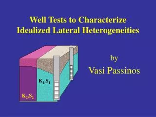
K 1 ,S 1. K 2 ,S 2. Well Tests to Characterize Idealized Lateral Heterogeneities. by Vasi Passinos and Larry Murdoch Clemson University. Faults. Steeply Dipping Beds. Facies Change. Marine Clay. Channel sand. Reef. Dike. Country rock. Batholith. Floodplain deposits.

E N D
K1,S1 K2,S2 Well Tests to Characterize Idealized Lateral Heterogeneities by Vasi Passinos and Larry Murdoch Clemson University
Faults Steeply Dipping Beds
Facies Change Marine Clay Channel sand Reef Dike Country rock Batholith Floodplain deposits Igneous Rocks
Local Neighboring T1S1 T2 S2=S1 L L Conceptual Models 2-Domain Model 3-Domain Model Region 1 Region 3 Strip T3 = T1 S3 = S1 T1 S1 T2 S2=S1 L w L
Methods • 2-Domain Model • Transient analytical solution using Method of Images (Fenske, 1984) • 3-Domain Model • Transient numerical model using MODFLOW • Tr and w of the strip were varied. • Grid optimized for small mass balance errors
2-Domain Model T Contrast Tr=10 Tr = 1 Tr=0.1
3-Domain Model T Contrast Tr = 10 Tr = 1 Tr = 0.1
Strip Transmissivness & Conductance • Hydraulic properties of the strip depend on strip conductivity and width • Strip is a higher K than matrix • Strip is a lower K than matrix
Well Graphical EvaluationBoundary Type and Location Low T to High T High T to Low T
Graphical EvaluationEstimate Aquifer Properties to=0.42 S=0.35 Ds=4.1 T = 0.55 to=0.029 S=0.017 Ds=2.3 T=1
Graphical EvaluationEstimate Aquifer Properties to = 2.7 S=0.136 Ds = 4.1 T=0.55
TL=0.55 SL=0.029 TL=0.55 SL=0.021 L TE=1 SE=0.0179 TL=0.55 SL=0.25 TE=1 SE=0.0179 TL=0.55 SL=0.136 TL=0.55 SL=0.27 TL=0.55 SL=0.068 TL=0.55 SL=0.06 TL=0.55 SL=0.021 L L
Graphical EvaluationEstimate Aquifer Properties to=0.09 S = 0.054 Ds = 2.3 T = 1 to=0.028 S = 0.017 Ds = 2.3 T = 1
Determine Properties of Strip • SSL analysis on the first line will give T and S of the area near the well. • Take the derivative of time and determine the maximum or minimum slope. • Using equations from curve fitting determine Tsd or Cd of the layer. • Solve for Tsor C
Field Case K.G. Fault
Field Case - Site Map BW2 BW-109 L
Determining Hydraulic Properties • Using Semi-Log Straight-Line Analysis : • Minimum slope using the derivative curve is 0.5 • Tsd=33.99=Ksw/KaL T = 0.053 ft2/min S = 2x10⁻⁴ ??? Ts = 23.79 ft2/min Ts/Ta = 450 L = 280 ft Distance to fault b = 21.5 ft screened thickness
Conclusions 2-Domain Model Semi-Log Straight-line Method • Piezometers r<0.3L gives T, S of local region. • Piezometers r>0.3L gives average T of both regions. • Piezometers r>0.3L unable to predict S • Piezometers in neighboring region also give average T of both regions. • Analyzing piezometers individually poor approach to characterizing heterogeneities.
Conclusions 3-Domain Model • Drawdown for low conductivity vertical layer controlled by conductance. C=Ks/w • Drawdown for high conductivity vertical layer controlled by strip transmissivness. Ts=Ks*w • Feasible to determine properties of a vertical layer from drawdown curves. • Drawdown curves non-unique. Require geological assessment.