Download

1 / 41
410 likes | 526 Vues
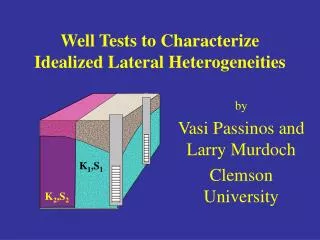
K 1 ,S 1. K 2 ,S 2. Well Tests to Characterize Idealized Lateral Heterogeneities. by Vasi Passinos. Faults. Steeply Dipping Beds. Facies Change. Floodplain deposits. Marine Clay. Channel sand. Reef. Dike. Country rock. Batholith. Igneous Rocks. Confined Aquifer.

E N D
K1,S1 K2,S2 Well Tests to Characterize Idealized Lateral Heterogeneities by Vasi Passinos
Faults Steeply Dipping Beds
Facies Change Floodplain deposits Marine Clay Channel sand Reef Dike Country rock Batholith Igneous Rocks
Confined Aquifer Unconfined Aquifer
Local Neighboring Matrix Matrix Strip T1S1 Tm Sm T2 S2 Tm Sm Ts Ss=Sm L w L L L Conceptual Models 2-Domain Model 3-Domain Model
Analysis Governing Equation Initial Condition Boundary Conditions when
1 2 L Analysis – 2-Domain • Conditions at the contact
m m s L w Analysis – 3-Domain • Conditions at the contact
Method – Analytical • Transient analytical solution using Method of Images (Fenske, 1984)
Methods – Numerical • Transient numerical model using MODFLOW • 2-Domain – Tr and Sr were varied • 3-Domain - Tr and w of the strip were varied. • Grid optimized for small mass balance errors • The properties of the model were selected so that the drawdown and time from the numerical model were dimensionless
Dimensionless Time • Drawdowns were evaluated at three dimensionless times to illustrate effects during development of drawdown fields. • Dimensionless time used for type curves • Dimensionless time used in drawdown fields
2-Domain Model T Contrast tdLA tdLC tdLB Tr=10 Tr = 1 Tr=0.1
2-Domain Model S Contrast tdLA tdLC tdLB Sr = 10 Sr = 1 Sr = 0.1
3-Domain Model T Contrast tdLB tdLC tdLD Tr = 10 Tr = 1 Tr = 0.1
to = 0.42 S = 0.35 Ds = 4.1 T = 0.55 to = 0.029 S = 0.017 Ds = 2.3 T = 1 Graphical Evaluation – 2-DomainEstimate Aquifer Properties
to = 2.7 S = 0.136 Ds = 4.1 T = 0.55 Graphical Evaluation – 2-DomainEstimate Aquifer Properties
TL=0.55 SL=0.029 TL=0.55 SL=0.021 L TE=1 SE=0.0179 TL=0.55 SL=0.25 TE=1 SE=0.0179 TL=0.55 SL=0.136 TL=0.55 SL=0.27 TL=0.55 SL=0.068 TL=0.55 SL=0.06 TL=0.55 SL=0.021 L L
Critical Region • An early semi-log straight line can be determined by • The second derivative was compared to plots with a variety of curves. An early SLSL could be identified by a second derivative of 0.2 or less from 0.3<tdL<2.5.
Critical Region • Observation points confined to a region that is within 0.3 to 0.5 of the distance between the pumping well and the linear discontinuity
Distance to the Contact Streltsova, 1988 tc = 7.3
Strip Transmissivness & Conductance • Hydraulic properties of the strip depend on strip conductivity and width • Strip K greater than matrix • Strip K less than matrix
to = 0.09 S = 0.054 Ds = 2.3 T = 1 to = 0.028 S = 0.017 Ds = 2.3 T = 1 Graphical Evaluation – 3-DomainEstimate Aquifer Properties
Determine Properties of Strip • SLSL analysis on the first line will give T and S of the area near the well. • Take the derivative of time and determine the maximum or minimum slope. • Using equations from curve fitting determine Tssd or Cd of the layer. • Solve for Tssor C
Non-Uniqueness Overlying Leaky Layer without storage Dual Porosity s Streltsova, 1988 Streltsova, 1984 Overlying Leaky Layer with storage Unconfined Aquifer w/delay yield from storage s Neuman, 1975 Streltsova, 1984 Log (t) Log (t)
Field Example stream N Up Down Ridge fault stream 500 feet
500 feet Field Case - Site Map Felsic N Mafic B-4 BW2 BW-109 L
Determining Hydraulic Properties Tm = 0.05 ft2/min Sm = 2x10⁻⁴ ??? • Using Semi-Log Straight-Line Analysis : • Minimum slope using the derivative curve is 0.5 • Tssd=34=Ksw/KaL • Tss = 24 ft2/min w = 10 to 20 ft Ts = 26 to 52 ft2/min Ts/Tm = 500 to 1000 L = 280 ft Distance to fault b = 21.5 ft screened thickness
Conclusions 2-Domain Model Using the Jacob method to analyze well tests: • Piezometers r < 0.25L gives T, S of local region. • Piezometers r > 0.25L gives average T of both regions. • Piezometers r > 0.25L unable to predict S
Conclusions – 2-Domain • Piezometers in neighboring region also give average T of both regions. • L can be determined from intersecting SLSLs using a piezometer within the critical region
Conclusions 3-Domain Model • Drawdown for low conductivity vertical layer controlled by conductance. C=Ks/w • Drawdown for high conductivity vertical layer controlled by strip transmissivness. Tss=Ks*w • Feasible to determine properties of a vertical layer from drawdown curves.
Conclusions • Analyzing piezometers individually is a poor approach to characterizing heterogeneities. • Drawdown curves non-unique. Require geological assessment.
Acknowledgments • Funding • Geological Society of America • Brown Foundation • National Science Foundation • Others…