Download
1 / 21
210 likes | 347 Vues
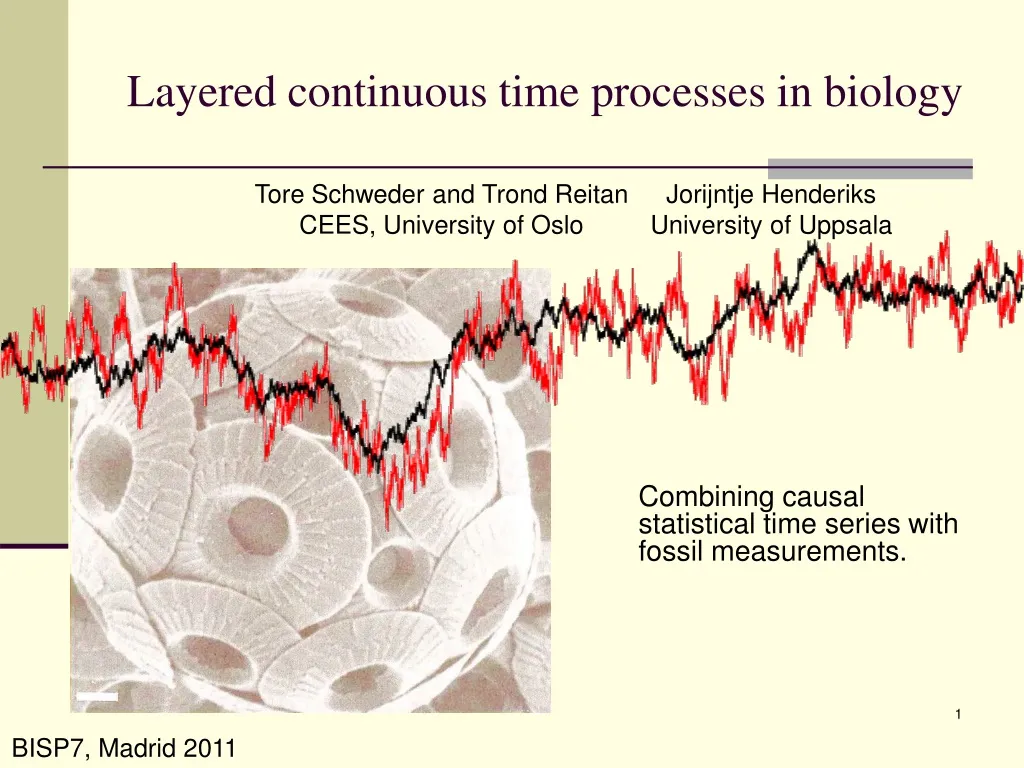
Layered continuous time processes in biology. Combining causal statistical time series with fossil measurements. Tore Schweder and Trond Reitan CEES, University of Oslo. Jorijntje Henderiks University of Uppsala. BISP7, Madrid 2011. Overview. Introduction - Motivating example:

E N D
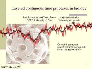
Layered continuous time processes in biology Combining causal statistical time series with fossil measurements. Tore Schweder and TrondReitan CEES, University of Oslo Jorijntje Henderiks University of Uppsala BISP7, Madrid 2011
Overview • Introduction - Motivating example: • Coccolith data (microfossils) • Phenotypic evolution: irregular time series related by (possibly common) latent processes • Causality in continuous time processes • Stochastic differential equation vector processes • Ito representation and diagonalization • Tracking processes and hidden layers • Kalman filtering • Model variants • Inference and results • Bayesian inference on model properties, models, process parameters and process states • Results for the coccolith data. • Second application: Phenotypic evolution on a phylogenetic tree • Primates - preliminary results • Conclusion
Irregular time series related by latent processes: evolution of body size in CoccolithusHenderiks – Schweder - Reitan • The size of a single cell algae (Coccolithus) is measured by the diameter of its fossilized coccoliths (calcite platelets). Want to model the evolution of a lineage found at six sites. • Phenotype (size) is a process in continuous time and changes continuously. 19,899 coccolith measurements, 205 sediment samples (1< n < 400) of body size by site and time (0 to -60 my).
Our data – Coccolith size measurements 205 Sample mean log coccolith size (1 < n < 400) by time and site.
Evolution of size distribution Fitness = expected number of reproducing offspring. The population tracks the fitness curve (natural selection) The fitness curve moves about, the population follow. With a known fitness, µ, the mean phenotype should be an Ornstein-Uhlenbeck process (Lande 1976). With fitness as a process, µ(t),, we can make a tracking model:
The Ornstein-Uhlenbeck process • Attributes: • Stationary • Normally distributed • long-term level: • Standard deviation: s=/2α • Markovian • α: pull • corr(x(0),x(t))=e-t • Time for the correlation to drop to 1/e: t =1/α The parameters (, t, s) can be estimated from the data. In this case: 1.99, t=1/α0.80Myr, s0.12. 1.96 s t -1.96 s
One layer tracking another Black process (t1=1/1=0.2, s1=2) tracking red process (t2=1/2=2, s2=1) Auto-correlation of the upper (black) process, compared to a one-layered SDE model. A slow-tracking-fast can always be re-scaled to a fast-tracking slow process. Impose identifying restriction: 1 ≥2
Process layers - illustration Observations Layer 1 – local phenotypic expression Layer 2 – local fitness optimum T External series Layer 3 – hidden climate variations or primary optimum Stationary expectancy
Causality in SDE processes We want to express in process terms the fact that climate affects the phenotypic optimum which again affects the actual phenotype. Local independence (Schweder 1970): • Context: Composable continuous time processes. • Component A is locally independent of B iff transition prob. of A does not depend on B. • If B is locally dependent on A but not vice versa, we write A→B. Local dependence can form a notion of causality in cont. time processes the same way Granger causality does for discrete time processes.
Stochastic differential equation (SDE) vector processes The zeros in this matrix determines the local independencies.
Model variants for Coccolith evolution Model variations: 1, 2 or 3 layers (possibly more) Inclusion of external time series or extra internal time series in connection to the one we are modelling In a single layer: Local or global parameters Correlation between sites (inter-regional correlation) Deterministic response to the lower layer Random walk (no tracking)
Likelihood: Kalman filter Need a linear, normal Markov chain with independent normal observations: Process Observations The Ito solution gives, together with measurement variances, what is needed to calculate the likelihood using the Kalman filter: and
Kalman smoothing (state inference)A tracking model with 3 layers and fixed parameters North Atlantic Red curve: expectancy Black curve: realization Green curve: uncertainty Snapshot:
Parameter and model inference • Wide but informative prior distributions respecting identifying restrictions • MCMC for parameter inference on individual models: • MCMC samples+state samples from Kalman smoother -> Possible to do inference on the process state conditioned only on the data. • Model likelihood (using an importance sampler) for model comparison (posterior model probabilities). • Posterior weight of a property C from model likelihoods:
Results • Best 5 models in good agreement. (together, 19.7% of summed integrated likelihood): • Three layers. • Common expectancy in bottom layer . • No impact of exogenous temperature series. • Lowest layer: Inter-regional correlations, 0.5. Site-specific pull. • Middle layer: Intermediate tracking. • Upper layer: Very fast tracking. Middle layers: fitness optima Top layer: population mean log size
Phenotypic evolution on a phylogenetic tree: Body size of primates
Why linear SDE processes? • Parsimonious: Simplest way of having a stochastic continuous time process that can track something else. • Tractable: The likelihood, L() f(Data | ), can be analytically calculated by the Kalman filter or directly by the parameterized multi-normal model for the observations. ( = model parameter set) • Can code for causal structure (local dependence/independence). • Some justification in biology, see Lande (1976), Estes and Arnold (2007), Hansen (1997), Hansen et. al (2008). • Great flexibility, widely applicable... • Thinking and modelling might then be more natural in continuous time. • Allows for varying observation frequency, missing data and observations arbitrary spaced in time. • Extensions: • Non-linear SDE models… • Non-Gaussian instantaneous stochasticity (jump processes).
Bibliography • Commenges D and Gégout-Petit A (2009), A general dynamical statistical model with causal interpretation. J.R. Statist. Soc. B, 71, 719-736 • Lande R (1976), Natural Selection and Random Genetic Drift in Phenotypic Evolution, Evolution 30, 314-334 • Hansen TF (1997), Stabilizing Selection and the Comparative Analysis of Adaptation, Evolution, 51-5, 1341-1351 • Estes S, Arnold SJ (2007), Resolving the Paradox of Stasis: Models with Stabilizing Selection Explain Evolutionary Divergence on All Timescales, The American Naturalist, 169-2, 227-244 • Hansen TF, Pienaar J, Orzack SH (2008), A Comparative Method for Studying Adaptation to a Randomly Evolving Environment, Evolution 62-8, 1965-1977 • Schuss Z (1980). Theory and Applications of Stochastic Differential Equations. John Wiley and Sons, Inc., New York. • Schweder T (1970). Decomposable Markov Processes. J. Applied Prob. 7, 400–410 Source codes, examples files and supplementary information can be found at http://folk.uio.no/trondr/layered/.