Download
1 / 19
190 likes | 320 Vues
Chapter Nine Inferences Based on Two Samples.

E N D
Hypothesis Test 2-Sample Means (Known )Both Normal pdf (known )Null Hypothesis: H0: u1 – u2 = 0Test Statistic: z = x – y – 0 21/m + 22/nAlternative Hypothesis:Reject RegionHa: u1–u2 > 0(Upper Tailed)z zHa: u1–u2 < 0 (Lower Tailed) z -zHa: u1–u2 0 (Two-Tailed) eitherz z/2 or z -z/2P-Value computed the same as 1-Sample Mean.
Example HT 2-Sample Means (Known )During a total solar eclipse the temperature drops quickly as the moon passes between the earth and the sun. During the June 2001 eclipse in Africa, data was collected on the drop in temperature in degrees F at two types of locations. The average drop in temperature for 9 samples taken in Mountainous terrain was 15.0. The average drop in temperature for 12 samples taken in River-level terrain was 17.5. Assume the variance in temperature drop is known to be 9 for this type of terrain-temperature drop experiment and that experiments of this type follow a Normal pdf. Is there evidence at the = .10 level to conclude that there is a difference in temperature drop between the two types of terrain in this experiment?P-value?
Determining ( known)Alternative Type IIHypothesisError ()Ha: u1 - u2 > 0 z- - 0 Ha: u1 - u2 < 0 1 - -z- - 0 Ha: u1 - u2 0 z/2-- 0 - -z/2- - 0 Where = X-Y = (21/m) + (22/n)
Example HT 2-Sample Means (Known )A study of report writing by student engineers was conducted at Watson School. A scale that measures the intelligibility of student engineers’ English is devised. This scale, called an “index of confusion,” is devised, to the delight of the students, so that low scores indicate high readability. Data are obtained on articles randomly selected from engineering journals and from unpublished reports. A sample of 16 engineering journals yielded an average score of 1.75 while a sample of 25 unpublished reports yielded an average score of 2.5. Variance for this type of scale is known to be 0.48 and the scores are known to follow a Normal pdf. At a significance level of .05, does there appear to be a difference between the average scores of the two types of reports? What is the Beta error when the true averages differ by as much as 0.5?
Hypothesis Test 2-Sample Means (Large n)Null Hypothesis: H0: u1 – u2 = 0Test Statistic: z = x – y – 0 s21/m + s22/nAlternative Hypothesis:Reject RegionHa: u1–u2 > 0(Upper Tailed)z zHa: u1–u2 < 0 (Lower Tailed) z -zHa: u1–u2 0 (Two-Tailed) eitherz z/2 or z -z/2Both m > 40 & n > 40.
Example HT 2-Sample Means (Large n)Aseptic packaging of juices is a method of packaging that entails rapid heating followed by quick cooling to room temperature in an air-free container. Such packaging allows the juices to be stored un-refrigerated. A new & old machine used to fill aseptic packages is being compared. The mean number of containers filled per minute on the new machine was 114.1 for 50 observations with a standard deviation of 5.0. The mean number of containers filled per minute on the old machine was 112.7 for 72 observations with a standard deviation of 3.0. Is there evidence that the new machine is faster than the old machine? Use a test with = .01. (Include the P-value).
Hypothesis Test 2-Sample Means (Small n)BothNormal pdf (unknown )Null Hypothesis: H0: u1 – u2 = 0Test Statistic: t = x – y – 0 s21/m + s22/nAlternative Hypothesis:Reject RegionHa: u1–u2 > 0(Upper Tailed)t t, Ha: u1–u2 < 0 (Lower Tailed) t -t, Ha: u1–u2 0 (Two-Tailed) eithert t/2, or t -t/2,
Estimating the Degrees of Freedoms21 + s222 = m n (s21/m)2 + (s22/n)2 m –1 n -1
Example HT 2-Sample Means (Small n)The slant shear test is used for evaluating the bond of resinous repair materials to concrete. The test utilizes cylinder specimens made of 2 identical halves bonded at 300C. Twelve specimens were prepared using wire brushing. The sample mean shear strength (N/mm2) and sample standard deviation were 19.20 & 1.58, respectively. Twelve specimens were prepared using hand-chiseled specimens; the corresponding values were 23.13 & 4.01.Does the true average strength appear to be different for the two methods of surface preparation? Use a significance level of .05 to test the relevant Hypothesis & assume the shear strength distributions to be Normal. (Include the P-value).Parameters of interest: R. R.:Null Hypothesis: Calculation:Alternative: Decision: Test Statistic: P-value:
Example HT 2-Sample Means (Small n)A manufacturer of power-steering components buys hydraulic seals from two sources. Samples are selected randomly from among the seals obtained from these two suppliers, and each seal is tested to determine the amount of pressure that it can withstand. These data result:Supplier I Supplier II x = 1342 lb/in2 y = 1338 lb/in2s2 = 100 s2 = 33 m = 10 n = 11Is there evidence at the = .05 level to suggest that the seals from supplier I can withstand higher pressures than those from supplier II? (P-value)Assume measurements of this type are Normal.
HT 2-Sample Means-Paired Data (Small n)BothNormal X and Y (unknown )Null Hypothesis: H0: uD= 0Test Statistic: t = d – 0sD / nAlternative Hypothesis:Reject RegionHa: uD > 0(Upper Tailed)t t, Ha: uD < 0 (Lower Tailed) t -t, Ha: uD 0 (Two-Tailed) eithert t/2, or t -t/2, D = X – Y within each paired observation.
Example HT 2-Sample Means-Paired Data (Small n)One important aspect of computing is the CPU time required by an algorithm to solve a problem. A new algorithm is developed to solve zero-one multiple objective problems in linear programming. It is thought that a new algorithm will solve problems faster than the algorithm currently used. To obtain statistical evidence to support this research hypothesis, a number of problems will be selected at random. Each problem will be solved twice; once using the current algorithm and once using the newly developed one. These CPU times are not independent; they are based on the same problems solved by two different methods and so are paired by design. The mean difference between the (16) paired data points was 2.7 seconds with a standard deviation calculated at 6.0 seconds. Does the data support this hypothesis at a = .025 level of significance? Assume measurements of this type are known to be Normal. (Give the P-value) Let X = old & Y = new.
Example HT 2-Sample Means-Paired Data (Large n)Highway engineers studying the effects of wear on dual-lane highways suspect that more cracking occurs in the travel lane of the highway than in the passing lane. To verify this contention, 64 one-hundred-feet-long test strips are selected, paved, and studied over a period of time. It is found that the mean difference in the number of major cracks is 3.3 with a sample deviation of 8.8. Does this data support the research hypothesis at a significance level of .05? (Include P-value). Let RV X = Travel lane & RV Y = Passing lane
The F Distribution = W/ = +/2 x(/2)-1 Y/ 2 x + 1 (+)/2 2 2 0 < x < W & Y are independent Chi-Square RV’s with & degrees of freedom.
Hypothesis Test on 2 Population VariancesBothNormal (unknown u1 & u2)Null Hypothesis: H0: 21= 22Test Statistic: = S21 / S22Alternative Hypothesis:Reject RegionHa: 21 > 22(Upper Tail) F, m-1, n-1Ha: 21 < 22(Lower Tail) F1- , m-1, n-1Ha: 21 22(Two-Tail) either F/2, m-1, n-1 or F1- /2, m-1, n-1F1- , m-1, n-1 = 1 / F, n-1, m-1 F-Tables pg. 730-735
Example HT 2-Population VariancesThe cost of repairing a fiberoptic component may depend of the stage of production at which it fails. The following data are obtained on the cost of repairing parts that fail when installed in the system and on the cost of repairing parts that fail after the system is installed in the field:System failureField failure Sample Size = 21 Sample Size = 25 Mean = $65 Mean = $120 s2 = 25 s2 = 100 It is thought that the variance in cost of repairs made in the field is larger than the variance in cost of repairs made when the component is placed into the system. Test at the = .10 level to see if there is statistical evidence to support this contention.
Example HT 2-Population VariancesOxide layers on semiconductor wafers are etched in a mixture of gases to achieve the proper thickness. The variability in the thickness of these oxide layers is a critical characteristic of the wafer, and low variability is desirable for subsequent processing steps. Two different mixtures of gases are being studied to determine whether one is superior in reducing the variability of the oxide thickness. Twenty wafers are etched in each gas. The sample standard deviation of oxide thickness are s1= 1.96 angstroms and s2= 2.13 angstroms, respectively. Is there any evidence to indicate that either gas is preferable? Use = 0.10 & assume measurements of this type are Normal.
Example HT 2-Population VariancesTwo companies supply raw materials to the manufacturer of paper products. The concentration of hardwood in these materials is important for the tensile strength of the products. The mean concentration of hardwood for both suppliers is the same; however, the variability in concentration may differ between the two companies. The standard deviation of concentration in a random sample of 26 batches produced by company X is 4.7 g/l, while for company Y a random sample of 21 batches yields 6.1 g/l. Is there sufficient evidence to conclude that the two population variances differ? Use = .05 & list any assumptions that you make.