Download
1 / 49
490 likes | 765 Vues
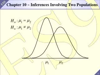
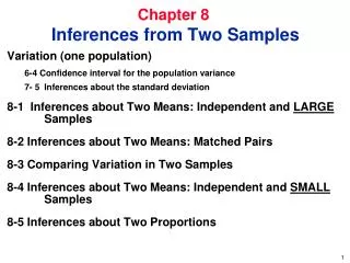
Inferences about Two Means: Independent and Large Samples Inferences about Two Means: Independent and Small Samples Inferences about Two Means: Matched Pairs Inferences about Two Proportions. Chapter 10 Inferences from Two Samples.

E N D
Inferences about Two Means: Independent and Large Samples Inferences about Two Means: Independent and Small Samples Inferences about Two Means: Matched Pairs Inferences about Two Proportions Chapter 10 Inferences from Two Samples
There are many important and meaningful situations in which it becomes necessary to compare two sets of sample data. Overview
10-2 Inferences about Two Means:Independent and Large Samples
Two Samples: Independent The sample values selected from one population are not related or somehow paired with the sample values selected from the other population. If the values in one sample are related to the values in the other sample, the samples are dependent. Such samples are often referred to as matched pairs or paired samples. Definitions
1. The two samples are independent. 2. The two sample sizes are large. That is, n1> 30 and n2> 30. 3. Both samples are simple random samples. Assumptions
The mean of the sampling distribution of all possible XA-XB is µA- µB. The standard deviation of the sampling distribution of all the possible values of Characteristics of theSampling Distribution XA-XB
Test Statistic for Two Means: Independent and Large Samples Hypothesis Tests
Test Statistic for Two Means: Independent and Large Samples Hypothesis Tests (x1- x2) - (µ1 - µ2) z= 1. 2 2 2 + n2 n1
Test Statistic for Two Means: Independent and Large Samples Hypothesis Tests and If and are not known, use s1 and s2 in their places. provided that both samples are large. P-value: Use the computed value of the test statistic z, and find the P-value . Critical values: Based on the significance level , find critical values .
Sample statistics are shown. Use the 0.01 significance level to test the claim that the mean weight of regular Coke is different from the mean weight of regular Pepsi. Coke Versus Pepsi
Sample statistics are shown. Use the 0.01 significance level to test the claim that the mean weight of regular Coke is different from the mean weight of regular Pepsi. Regular Coke Regular Pepsi n 36 36 x 0.81682 0.82410 s 0.007507 0.005701 Coke Versus Pepsi
Claim: 12 Ho : 1 = 2 H1 : 12 = 0.01 Coke Versus Pepsi Fail to reject H0 Reject H0 Reject H0 Z = - 2.575 Z = 2.575 1 - = 0 or Z = 0
Test Statistic for Two Means: Independent and Large Samples (x1- x2) - (µ1 - µ2) z= 1. 2 2 2 + n2 n1 Coke Versus Pepsi
Test Statistic for Two Means: Independent and Large Samples Coke Versus Pepsi (0.81682 - 0.82410) - 0 z= 0.005701 2 0.0075707 2 + 36 36 = - 4.63
Claim: 12 Ho : 1 = 2 H1 : 12 = 0.01 Coke Versus Pepsi Reject H0 Reject H0 Fail to reject H0 Z = - 2.575 Z = 2.575 1 - = 0 or Z = 0 sample data: z = - 4.63
Claim: 12 Ho : 1 = 2 H1 : 12 = 0.01 Coke Versus Pepsi There is significant evidence to support the claim that there is a difference between the mean weight of Coke and the mean weight of Pepsi. Reject H0 Reject H0 Fail to reject H0 Reject Null Z = - 2.575 Z = 2.575 1 - = 0 or Z = 0 sample data: z = - 4.63
Confidence Intervals (x1- x2) - E < (µ1 - µ2) < (x1- x2) + E
Confidence Intervals (x1- x2) - E < (µ1 - µ2) < (x1- x2) + E 2 1 2 2 whereE = z + n2 n1
(x1- x2) - E < (µ1 - µ2) < (x1- x2) + E whereE = z 2 1 2 2 + n2 n1 For Coke versus Pepsi, x1- x2 = .00728, and z =1.28 Confidence Intervals Find an 80% confidence interval for the difference for Coke and Pepsi. .00728 + 1.28(.00157) = (.00527, .00929)
(x1- x2) - (µ1 - µ2) t= 1. 2 2 2 + n2 n1 t-Distribution Model • The degrees of freedom are nA+ nB – 2 • A pooled variance is the weighted mean of the sample variances. • and is used if the the data is not normally distributed.
Two groups were tested to see whether calcium reduces blood pressure. The following data was collected. Is there evidence at the .1 level that calcium reduces blood pressure? Group 1 (calcium) 7 -4 18 17 -3 -5 1 10 11 –2 Group 2 (placebo) -1 12 -1 -3 3 -5 5 2 -11 -1 -3 Group Treatment n x s 1 Calcium 10 5.00 8.743 2 Placebo 11 -.273 5.901 • HO: µ1 - µ2 > 0 • HA: µ1 - µ2 < 0 3. tcritical = -1.328 • One tail t test, n < 30 • 11 + 10 – 2 = 19 d.f.
5. There is not enough evidence at the .1 level that calcium reduces blood pressure. -1.328 1.604
Assumptions 1. We have proportions from two independent simple random samples. 2. For both samples, the conditions np 5 and nq 5 are satisfied. Inferences about Two Proportions
For population 1, we let: p1 = population proportion n1 = size of the sample x1 = number of successes in the sample Notation for Two Proportions
For population 1, we let: p1 = population proportion n1 = size of the sample x1 = number of successes in the sample Notation for Two Proportions ^ p1 = x1/n1 (the sample proportion)
For population 1, we let: p1 = population proportion n1 = size of the sample x1 = number of successes in the sample Notation for Two Proportions ^ p1 = x1/n1 (the sample proportion) q1 = 1 - p1 ^ ^
For population 1, we let: π1 = population proportion n1 = size of the sample x1 = number of successes in the sample Notation for Two Proportions p1 = x1/n1 (the sample proportion) q1 = 1 - p1 The corresponding meanings are attached to π2, n2 , x2 , p2. and q2 , which come from population 2.
For H0: π1 = π2 , H0: π1 π2 , H0: π1π2 HA:π1 π2 , HA: π1 <π2 , HA: π1> π2 Test Statistic for Two Proportions
For H0: p1 = p2 , H0: p1 p2 , H0: p1p2 H1: p1 p2 , H1: p1 < p2 , H1: p 1> p2 Test Statistic for Two Proportions whereπ1 - π2 = 0 (assumed in the null hypothesis)
For H0: p1 = p2 , H0: p1 p2 , H0: p1p2 H1: p1 p2 , H1: p1 < p2 , H1: p 1> p2 Test Statistic for Two Proportions wherep1 - p 2 = 0 (assumed in the null hypothesis) x2 x1 p1 p2 and = = n1 n2
(p1 - p2 ) - E < (π1 - π2 ) < (p1 - p2 ) + E Confidence Interval Estimate of π1 - π2 If 0 is not in the interval, one may be C% confident that the two population proportions are different.
A sample of households in urban and rural homes displayed the following data for preference of artificial or natural Christmas trees: Population n X p = X/n 1(urban) 261 89 .341 2(rural 160 64 .400 Is there a difference in preference between urban and rural homes? with a confidence interval of 90%?
(-.139, .021) We are 90% confident that the difference in proportions is between -.14 and .02. Because the interval contains 0, we are not confident that either group has a stronger preference for natural trees than the other group.
1. The sample data consist of matched pairs. 2. The samples are simple random samples. 3. If the number of pairs of sample data is small (n 30), then the population of differences in the paired values must be approximately normally distributed. Assumptions
Notation for Matched Pairs µd= mean value of the differences d for the population of paired data
sd= standard deviation of the differences d for the paired sample data n = number of pairs of data. Notation for Matched Pairs µd= mean value of the differences d for the population of paired data d = mean value of the differences d for the paired sample data (equal to the mean of the x - y values)
Test Statistic for Matched Pairs of Sample Data d- µd t= sd n where degrees of freedom = n - 1
Critical Values If n 30, critical values are found in Table A-4 (t-distribution). If n > 30, critical values are found in Table A- 2 (normal distribution).
Confidence Intervals d -ME < µd < d + ME
degrees of freedom =n-1 Confidence Intervals d -ME < µd < d + ME sd where ME =t n
Using the sample data from Table 8-1 with the outlier excluded, construct a 95% confidence interval estimate of d, which is the mean of the differences between reported heights and measured heights of male statistics students. How Much Do Male Statistics Students Exaggerate Their Heights?
Reported and Measured Heights (in inches) of Male Statistics Students Student A B C D E F G H I J K L Reported 68 74 82.25 66.5 69 68 71 70 70 67 68 70 Height Measured 66.8 73.9 74.3 66.1 67.2 67.9 69.4 69.9 68.6 67.9 67.6 68.8 Height Difference 1.2 0.1 7.95 0.4 1.8 0.1 1.6 0.1 1.4 -0.9 0.4 1.2
d = 1.279 s = 2.243 n = 12 t = 2.201 (found from Table A-3 with 11 degrees of freedom and 0.05 in two tails) How Much Do Male Statistics Students Exaggerate Their Heights?
sd n How Much Do Male Statistics Students Exaggerate Their Heights? E = t E = (2.201)( ) 2.244 12 = 1.426
How Much Do Male Statistics Students Exaggerate Their Heights? 1.279 - 1.464 < µd< 1.279 + 1.464 In the long run, 95% o f such samples will lead to confidence intervals that actually do contain the true population mean of the differences. Since the interval does contain 0, the true value of µdis not significantly different from 0. There is not sufficient evidence to support the claim that there is a difference between the reported heights and the measured heights of male statistics students.