Download
1 / 1
10 likes | 129 Vues
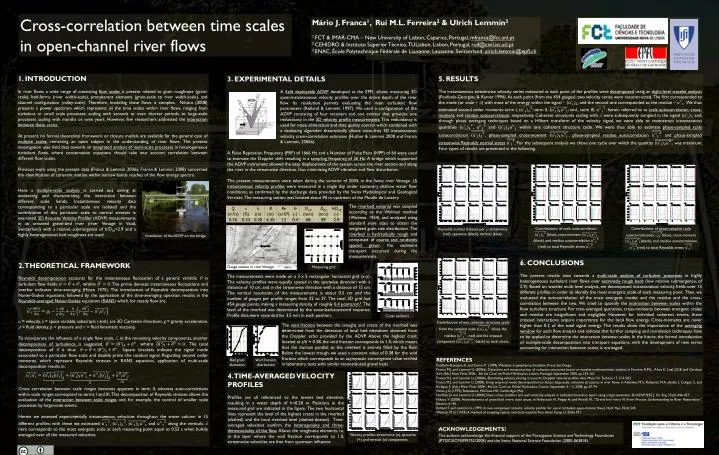
Cross-correlation between time scales in open-channel river flows. Mário J. Franca 1 , Rui M.L. Ferreira 2 & Ulrich Lemmin 3 1 FCT & IMAR-CMA – New University of Lisbon , Caparica , Portugal, mfranca@fct.unl.pt

E N D
Cross-correlation between time scales in open-channel river flows Mário J. Franca1, Rui M.L. Ferreira2 & Ulrich Lemmin3 1 FCT & IMAR-CMA – New UniversityofLisbon, Caparica, Portugal, mfranca@fct.unl.pt 2 CEHIDRO & Instituto Superior Técnico, TULisbon, Lisbon, Portugal, ruif@civil.ist.utl.pt 3 ENAC, École Polytechnique Fédérale de Lausanne, Lausanne, Switzerland, ulrich.lemmin@epfl.ch 1. INTRODUCTION In river flows a wide range of coexisting flow scales is present related to grain roughness (grain-scale), bed-forms (river width-scale), protuberant elements (grain-scale to river width-scale), and channel configuration (valley-scale). Therefore, modeling these flows is complex. Nikora(2008) presents a power spectrum which represents all the time scales within river flows, ranging from turbulent or small scale processes, scaling with seconds or even shorter periods, to large-scale processes scaling with months or even years. However, few researchers addressed the interaction between these scales. At present, no formal theoretical framework or closure models are available for the general case of multiple scales, remaining an open subject in the understanding of river flows. The present investigation uses field data towards an integrated analysis of multi-scale processes in heterogeneous turbulent flows, where conservation equations should take into account correlation between different flow scales. Previous work using the present data (Franca & Lemmin 2006a; Franca & Lemmin 2008) concerned the identification of coherent motion within narrow bands reaches of the flow energy spectra. 5. RESULTS The instantaneous streamwise velocity series measured at each point of the profiles were decomposed using an eight-level wavelet analysis (Foufoula-Georgiou & Kumar 1994). At each point (from the 454 gauges), two velocity series were reconstructed. The first corresponded to the mode (or scale – l) with most of the energy within the signal – , and the second one corresponded to the residue – . We thus estimated second order moments: term I, ;term II, ; and , term III, ; herein referred to as scale autocorrelation, cross-moment, and residue autocorrelation, respectively. Coherent structures scaling with lwere subsequently sampled in the signal and, through phase averaging techniques based on a Hilbert transform of the velocity signal, we were able to reconstruct instantaneous quantities , and within one coherent structure cycle. We were thus able to estimate phase-sampled scale autocorrelation, phase-sampled cross-moment, phase-sampled residue autocorrelation and phase-sampled streamwise Reynolds normal stress. For the subsequent analysis we chose one cycle over which the quantity was maximum. Four types of results are presented in the following. 3. EXPERIMENTAL DETAILS A field deployable ADVP developed at the EPFL allows measuring 3D quasi-instantaneous velocity profiles over the entire depth of the river flow. Its resolution permits evaluating the main turbulent flow parameters (Rolland & Lemmin 1997). We used a configuration of the ADVP consisting of four receivers and one emitter that provides one redundancy in the 3D velocity profile measurements. This redundancy is used for noise elimination and data quality control which combined with a dealiasing algorithm theoretically allows noise-free 3D instantaneous velocity cross-correlation estimates (Huther & Lemmin 2000 and Franca & Lemmin, 2006b). A Pulse Repetition Frequency (PRF) of 1666 Hz and a Number of Pulse Pairs (NPP) of 64 were used to estimate the Doppler shift, resulting in a sampling frequency of 26 Hz. A bridge which supported the ADVP instrument allowed the easy displacement of the system across the river section and along the river in the streamwise direction, thus minimizing ADVP vibration and flow disturbance. The present measurements were taken during the summer of 2004, in the Swiss river Venoge. 15 instantaneous velocity profileswere measured in a single day under stationary shallow water flow conditions, as confirmed by the discharge data provided by the Swiss Hydrological and Geological Services. The measuring station was located about 90 m upstream of the Moulin de Lussery. Here a multiple-scale analysis is carried out aiming at evidencing and characterizing the interaction between different scale bands. Instantaneous velocity data corresponding to a particular scale are isolated and the contribution of this particular scale to normal stresses is examined. 3D Acoustic Velocity Profiler (ADVP) measurements in an armored gravel-bed river (river Venoge in Vaud, Switzerland) with a relative submergence of h/D50=2.9 and a highly heterogeneous bed roughness are used. The riverbed material was sampled according to the Wolman method (Wolman, 1954), and analyzed using standard sieve sizes to obtain the weighted grain size distribution. The riverbed is hydraulically rough and composed of coarse and randomly spaced gravel. No sediment transport occurred during the measurements. Contributions of scale autocorrelation (blue), cross-moment (black), and residue autocorrelation (red) to total Reynolds stress . Contributions of phase-sampled scale autocorrelation(blue), cross-moment (black), and residue autocorrelation (red) to total Reynolds stress . Reynolds normal stresses per r: streamwise(red), spanwise(black), vertical (blue). Installation of the ADVP on the bridge 6. CONCLUSIONS The present results aims towards a multi-scale analysis of turbulent processes in highly heterogeneous turbulent river flows over extremely rough beds (low relative submergence, of 2.9). Based on wavelet multi-level analysis, we decomposed instantaneous velocity fields over 15 different profiles in order to identify the most energetic scale of each measuring point. Then, we evaluated the autocorrelation of the most energetic modes and the residue and the cross-correlation between the two. We tried to quantify the interaction between scales within the flow turbulent structure. For time-averaged quantities, cross-moments between energetic scales and residue are insignificant and negligible. However, for individual coherent events, these crossed interactions acquire importance for the local flow energy. Cross-moments are never higher than 0.2 of the total signal energy. The results show the importance of the averaging window for each flow analysis and indicate that further sampling and correlation techniques have to be applied to determine the interaction between scales. In the future, the formal introduction of multiple-scale decomposition into transport equations, with the development of new terms accounting for interaction between scales, is envisaged. 2. THEORETICAL FRAMEWORK Reynolds decomposition accounts for the instantaneous fluctuation of a generic variable qin turbulent flow fields:, where The prime denotes instantaneous fluctuations and overbarindicates time-averaging (Hinze 1975). The introduction of Reynolds decomposition into Navier-Stokes equations, followed by the application of the time-averaging operator, results in the Reynolds-averaged Navier-Stokesequations (RANS) which, for steady flow are: u = velocity, x = space variable; subscripts i and j are 3D Cartesian directions, g = gravity acceleration, r = fluid density, p = pressure and n = fluid kinematic viscosity. To incorporate the influence of a single flow scale, l, in the remaining velocity components, anotherdecomposition of turbulence is suggested, , where . The total decomposition of qis thus: . Square brackets indicate the signal mode associated to a particular flow scale and double prime the residual signal. Regarding second order moments, which represent Reynolds stresses in RANS equations, application of multi-scale decomposition results in: Cross correlation between scale ranges becomes apparent in term II, whereas auto-correlations within scale ranges correspond to terms I and III. This decomposition of Reynolds stresses allows the evaluation of the interaction between scale rangesand, for example, the control of smaller scale processes by large-scale events. Herein we assessed experimentally instantaneous velocities throughout the water column in 15 different profiles; with these we estimated: , , and along the verticals. l here corresponds to the most energetic scale at each measuring point equal to 0.53 s when bulkily averaged over all the measured velocities. Gauge station in river Venoge Measuring grid The measurements were made on a 3 x 5 rectangular horizontal grid (x-y). The velocity profiles were equally spaced in the spanwise direction with a distance of 10 cm, and in the streamwise direction with a distance of 15 cm. The vertical resolution of the measurements is about 0.5 cm and the number of gauges per profile ranges from 22 to 37. The total 3D grid had 454 gauge points, making a measuring density of roughly 0.4 points/cm3. The level of the riverbed was determined by the sonar-backscattered response. Profile data were recorded for 3.5 min in each position. Cross sections Contribution of one coherent structure cycle from the sampled scale ( ; blue), the residue (; red) and the crossed component ( ; black) to total stress. The void fraction between the troughs and crests of the riverbed was determined from the detection of local bed elevations obtained from the Doppler echo provided by the ADVP. Above the highest crest, located at z/h ≈ 0.38, the void fraction corresponds to 1.0, which means that the domain parallel to the riverbed is entirely filled by the fluid. Below the lowest trough, we used a constant value of 0.38 for the void fraction which corresponds to an asymptotic convergence value verified in laboratory tests with similar reconstituted gravel beds. REFERENCES Foufoula-Georgiou E. and Kumar P. (1994), Wavelets in geophysics, Academic Press, San Diego. Franca M.J. and Lemmin U. (2006a), Detection and reconstruction of coherent structures based on wavelet multiresolution analysis, in Ferreira R.M.L., Alves E., Leal, J.G.B. and Cardoso A.H. (Eds) River Flow 2006 - 3th Int. Conf. on Fluvial Hydraulics, Lisbon, Portugal, September 2006, pp.153-162. Franca M.J. and Lemmin U. (2006b), Eliminating velocity aliasing in acoustic Doppler velocity profiler data, Meas. Sci. Technol. 17, 313-322. Franca M.J. and Lemmin U. (2008), Using empirical mode decomposition to detect large-scale coherent structures in river flows, in Altinakar, M.S., Kokpinar, M.A., Aydin, I., Cokgor, S., and Kirkgoz, S. (Eds.) River Flow 2008 - 4th Int. Conf. on Fluvial Hydraulics, Cesme, September 3 – 5, 2008, pp. 67-74. Hinze, J.O. (1975), Turbulence, McGraw-Hill, Cambridge (Ma). HurtherD. and Lemmin U. (2000), Shear stress statistics and wall similarity analysis in turbulent boundary layers using a high-resolution 3D ADVP, IEEE J. Oc. Eng. 25(4): 446-457. NikoraV. (2008), Hydrodynamics of gravel-bed rivers: scale issues, in Habersack H., Piegay H. and Rinaldi M., “Gravel-bed rivers VI: From Process Understanding to River Restoration”, Elsevier, 61-81. Rolland T. and Lemmin U. (1997), A two-component acoustic velocity profiler for use in turbulent open-channel flow, J. Hydr. Res. 35(4) 545. Wolman M.G. (1954), A method of sampling coarse river-bed material, Tran. Amer. Geop. U. 35(6) 951. Bed grain diameters Void fraction distribution 4. TIME-AVERAGED VELOCITY PROFILES Profiles are all referenced to the lowest bed elevation, resulting in a water depth of h=0.20 m. Positions in the measured grid are indicated in the figure. The two horizontal lines represent the level of the highest crests in the riverbed (dashed) and the local riverbed level (dashed-dotted). Time-averaged velocities confirm the heterogeneity and three-dimensionality of the flow. Above the roughness elements, i.e. in the layer where the void fraction corresponds to 1.0, streamwise velocities are free from upstream influence. ACKNOWLEDGEMENTS: The authors acknowledge the financial support of the Portuguese Science and Technology Foundation (PTDC/ECM/099752/2008) and the Swiss National Science Foundation (2000-063818). Velocity profiles: streamwise(x), spanwise (+) and vertical (o) components.