Download
1 / 38
400 likes | 434 Vues
Remote Sensing of Energy Balance Fluxes. Net Radiation Albedo and Surface Emissivity Sensible Heat Fluxes Latent Heat Fluxes. Net Radiation. The amount of energy at the surface available to do work. It results from the balance of short wave and long wave radiation at the surface.

E N D
Remote Sensing of Energy Balance Fluxes Net Radiation Albedo and Surface Emissivity Sensible Heat Fluxes Latent Heat Fluxes
Net Radiation • The amount of energy at the surface available to do work. It results from the balance of short wave and long wave radiation at the surface. Rn = Rsin – Rsout + RLin – RLout Where Rn is the net radiation, Rsin is the incoming total solar radiation, Rsout is the reflected or outgoing solar radiation, RLin is the incoming longwave radiation from the atmosphere and RLout is the outgoing longwave radiation emitted by the surface. • Net radiation is partitioned and used by different processes at the surface. Rn = LE + H + G + P + ΔS • Where LE is the latent heat flux, H is the sensible heat flux and G is the soil heat flux, P is energy used in photosynthesis and ΔS is the energy stored, such as from a very dense and tall vegetation canopy.
Net Radiation • Photosynthesis and storage are very small terms relative to the other components and can usually be ignored, reducing the energy balance equation to: Rn = LE + H + G • LE is the latent heat flux or evapotranspiration, or energy used to evaporate water • H is the sensible heat flux or energy used to heat the air • G is the soil heat flux or energy used to heat the soil Rn, H and G can be estimated using remotely sensed inputs
Net Radiation • Is the balance of short wave and long wave radiation at the surface which provides energy to do work
Net Radiation • The balance of short wave and long wave radiation at the surface can be re-written as: Rn = (1 - α) Rsin + RLin – RLout Where α is the total reflectance of the surface in the shortwave spectrum, called albedo. Rsincan be measured at the surface using pyranometers. RLin = εaσ Ta • Where εais the emissivity of the air, σ is the Stefan-Bolzman constant (5.67x10⁻⁸ Watts/m2/K4),and Ta is the temperature of the air (K). RLout = εsurfσ Tsurf • Where εsurfis the emissivity of the surface, σ is the Stefan-Bolzman constant (5.67x10⁻⁸ Watts/m2/K4),and Tsurf is the temperature of the surface (K).
Albedo • Albedo αis the total reflectance of a surface in the shortwave part of the spectrum. It can be estimated using spectral-radiometers, or estimated from single band radiometers or satellite sensors through different methods such as the Brest and Goward (1987) or the P/T (partial/total) method.
Net Radiation • If the emissivity of the surface is low, then an additional turn to take into account the surface reflectivity term must be included: Rn = (1 - α) Rsin + εaσ Ta – εsurfσ Tsurf – (1 - εsurf ) * εaσ Ta • The emissivity of the air εacan be estimated from the Brutsaert (1975) equation: Εa = 1.24 (ea / Ta )1/7 Where ea is the vapor pressure (mb) and Ta is the temperature of the air (°C).
Emissivity of the Surface • Surface emissivity in the thermal infrared part of the spectrum varies according to the material: Fully grown and dense vegetation: 0.97-0.98 Dry bare soil: 0.90 (sand), 0.92-0.94 (clay, depending on color) Asphalt: 0.95- 0.97 (dry), 1.0 (wet) Polished metals: 0.16 – 0.21 Aluminum foil: 0.05 Granite: 0.86 Concrete: 0.70 – 0.90 depending on coloring and roughness Water: 0.92-0.98 (depending on sediment concentration) For vegetated scenes with mixed densities and cover, the surface emissivity can be estimated by scaling between bare soil and full cover vegetation according to the fraction of vegetation cover. For such different methods have been proposed.
Fraction of Cover • One method was proposed by Brunsell and Gillies (2002), PE&RS: • The method scales the NDVI to obtain the fraction of vegetation cover and then scales the fraction between the emissivity of bare soil and a full canopy: N* = (NDVI – NDVI0)/(NDVImax – NDVI0) Where NDVI0 is the bare soil NDVI value of the scene and NDVImax is the maximum NDVI of the scene corresponding to full cover dense vegetation. The fraction of cover becomes: Fr = N*2 The scaling of the surface emissivity is done using: εsurf = Fr (εveg ) + (1 – Fr) εsoil
Soil Heat Flux • Soil heat flux is the portion of the net radiation entering the soil matrix. It is a function of the vegetation cover (shading), soil moisture and the heat capacity of the soil. • Using remotely sensed inputs it can be calculated as a fraction of the net radiation using a vegetation index such as the NDVI to modulate the plant cover Jackson et al, (1987), working with wheat canopies proposed: G = 0.583 e(-2.13NDVI) Rn Bastiaansen (2000) proposed, used in the SEBAL model: G/Rn = Ts/α (0.0038α + 0.0074α2)(1 - .98NDVI4) • Chavez, Neale et al (2005) estimated G as a function of leaf area index (LAI) for corn and soybean canopies in Iowa: G = {[(0.3324 + (-0.024 * LAI)) * (0.8155+(- 0.3032 * LN (LAI)))] * Rn} LAI = (4 * OSAVI – 0.8)* (1 + 4.73E-6 * e [15.64 * OSAVI])
Sensible Heat Flux • This is the most complicated term to obtain from remote sensing. H = a Cpa (Taero – Ta) / rah Where a is the density of the air (kg m-3), Cpa is specific heat of air (J kg-1 K-1).,Ta is average air temperature, [K]. Taero is average surface aerodynamic temperature, (K) defined for a uniform surface as the temperature at the height of the zero plane displacement plus the roughness length (d+Zoh) for sensible heat transfer Zoh (m). This term is difficult to measure. For full canopies, it has been substituted in the past with Tc, the canopy temperature. Taero can be obtained empirically as a function of surface temperature, air temperature and LAI, such as the equation proposed by Chavez, Neale et al, (2005): Taero_e = [(0.534 Ts_RS) + (0.39 Ta) + (0.224 LAI_RS) – (0.192 U) + 1.67] Where Ts and LAI are obtained spatially through remote sensing and air temperature (Ta) and winds peed (U) are measured on the ground.
G alfalfa = (038 * EXP [-1.65 * NDVI]) * Rn Chavez et al, (2005) Neale et al, (2005) One Layer Energy Balance Model LE = Rn - G - H Brest and Goward (1987) Brutsaert (1975); Crawford and Duchon, 1999 LAI_air = (4 * OSAVI – 0.8)* (1 + 4.73E-6 * EXP [15.64 * OSAVI])1 LAI_sat = (2.88 * NDWI + 1.14)* (1 + 0.104 * EXP [4.1 * NDWI])1 L = 0.16 Gcorn, soy = {[(0.3324 + (-0.024 LAI)) (0.8155 + (- 0.3032 ln (LAI)))] Rn} hc_CORN air = (1.86 * OSAVI – 0.2)* (1 + 4.82E-7 * EXP [17.69 * OSAVI])1 hc_SOY air = (0.55 * OSAVI – 0.02)* (1 + 9.98E-5 * EXP [9.52 * OSAVI])1 Taero= [(0.534 Ts_RS) + (0.39 Ta) + (0.224 LAI_RS) – (0.192 U) + 1.67] hc_CORN sat = (1.20 NDWI + 0.6) (1 + 4.00E-2 EXP [5.3 NDWI])1 hc_SOY sat= (0.5 NDWI + 0.26) (1 + 5.0E-3 EXP [4.5 NDWI]) 1 Chavez et al, (2005) H = a Cpa (Taero – Ta) / rah Ground Measured Data [Ta, U, Rs] 1Anderson, M.C., C.M.U. Neale, F. Li, J.M. Norman, W. P. Kustas, H. Jayanthi, and J. Chavez, (RSE Vol. 92, pp. 447-4642004)
Surface Aerodynamic Resistance (rah) Iterative Procedure based on the Monin-Obukhov Method Zom = 0.123 hc Zoh = 0.1 Zom d = 0.67 hc H = a Cpa (Taero – Ta) / rah Taero_RS If rah_i-1 = rah_i
Sensible Heat Flux The empirical methodology is difficult to implement for sparse and non-uniform canopies, for example natural vegetation found in semi-arid regions. In such situations, another approach is needed to obtain sensible heat fluxes, by estimating the heat flux generated by the canopy and soil separately. One model is the Two-source model by Norman et al, (1995), Li et al, (2005). A third approach proposed by Bastiaansen (2000) is the SEBAL model (surface energy balance model) to be used with Landsat satellite imagery. He proposes selecting a “wet” and a “dry” pixel in the image to calculate a dT (temperature difference) using the thermal IR band, by passing the need for estimating the Taero term. (OBS: More details on these models and approaches can be given on request)
Norman et al (1995) Kustas and Norman (1999) Li et al, (2005) Two-source Model TR (φ) = {fc (φ) TC4 + [1- f (φ)] TS4}1/4 Hc = ρCp (Tc – Ta) / rah H = Hc + Hs Hs = ρCp (Ts – Ta) / (rah + rs) rs = 1 / (a + b us) LE = LEc + LEs
Reflectance-based Crop Coefficient Model (Kcrf) Neale et al (1989) Bausch (1993) Jayanthi et al, (2000, 2007) • ETc = Kc . ETr ETr is daily reference evapotranspiration Kc is the crop coefficient • Kc = Kcb.Ks + Ke Kcb is the basal crop coefficient for no limiting water in root zone and dry soil surface Ke is the adjustment for wet soil surface Ks is the adjustment for limited moisture in the root zone • Kcb = Kcrf => f(SAVI, NDVI) Crop coefficient curves can be represented by polynomial or linear functions
Example of Application SMACEX Experiment in Iowa Summer of 2002 Rainfed Corn and Soybean cropped area Measured fluxes with 13 eddy covariance flux stations Remote sensing from satellite (LANDSAT TM) and USU aircraft
Spatially Distributed Leaf Area Index, Canopy Height, Fraction of Vegetation Cover Leaf Area Index: Airborne (1.5 meter) Satellite (30 meter) Anderson, Neale, Li, Norman, Kustas, Jayanthi, and Chavez, 2004. Remote Sensing of Environment, 92, 447-464.
Latent Heat Flux Instantaneous R.S. LE to daily ET LE = Rn – G – H ETd = [EF (Rn – G)d] x [cf / v w] EF = LEi / (Rn – G)i ETd = Daily or 24 hours evapotranspiration rate, mm d-1 (Rn – G)d = Measured mean 24 hr available energy, W m-2 cf = Time (unit) conversion factor equal to 86400 s d-1, v = Latent heat of vaporization, W s kg-1 w = Density of Water, kg m-3
Study Area: Corn and Soybean Fields (Ames, Iowa)2002 NASA SMACEX – SMEX02 LANDSAT Thematic Mapper Image of study area: 30 meter resolution July 1st (182). Images also available for June 23rd, July 8th, July 16,17
Analysis upwind rectangles for averaging the estimated energy balance fluxes
LANDSAT Thermal Infrared Imagery Calibrated using MODTRAN Atmospheric Transmission Model and adjusted for surface emmissivity to obtain at-surface temperatures Berk et al (1989) Brunsel and Gillies (2002)
Energy balance fluxes measured with 11 eddy covariance systems (full energy balance) placed in the corn and soybean fields Corn Soybean 4 sets of soil heat flux plates distributed in rows and furrows
Modeling Environment (SETMI) Application code written in Visual Basic within ArcGIS 9.1
Results Spatial Output: Regional Daily ET on July 1, 2002(Spatial Model Output using the OLEM) Actual ET (mm/day)
Results: Net RadiationIntegrated over the upwind footprint Fields 15 & 16, July 1 & July 8 overpasses MBE = - 4.8 W m-2 RMSE = 20.7 W m-2
Results: Energy Balance Models (closure forced with the residual method) Sensible Heat Flux (H)
Latent Heat Fluxes High resolution multispectral High resolution coarsened Landsat Thematic Mapper 7 1.5 m shortwave, 6 m thermal to 30 m 30 m shortwave 60 m thermal from the USU airborne system Corn Soybean
Daily Evapotranspiration Integrated Using the Evaporative Fraction
Final Thoughts • The visual basic application is fast and allows for easy model integration. The ArcGIS environment allows for display and visual interpretation of results. • Energy balance models tested provide good estimates of latent heat fluxes • Thermal infrared band very important for estimating plant-soil water condition • High-resolution thermal is necessary in agricultural areas where scale of variability is considerable