Download

1 / 24
250 likes | 465 Vues
Chapter 3. Interpolation and Extrapolation. Hui Pan, Yunfei Duan. possible problem in physical measurement . Sometimes know the value of a function f(x) at a set of points, but we don’t have an analytic expression for f(x) that lets us calculate its value at an arbitrary point. .

E N D
Chapter 3. Interpolation and Extrapolation Hui Pan, YunfeiDuan
possible problem in physical measurement Sometimes know the value of a function f(x) at a set of points, but we don’t have an analytic expression for f(x) that lets us calculate its value at an arbitrary point.
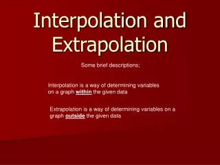
Interpolation and Extrapolation Estimate f(x) for arbitrary x by, in some sense, drawing a smooth curve through the xi. If the desired x is in between the largest and smallest of the xi’s the problem is called interpolation. Otherwise it is called extrapolation.
For example, suppose we have a table like this, which gives some values of an unknown function f. Interpolation provides a means of estimating the function at intermediate points, such as x = 2.5.1 1: from wiki: http://en.wikipedia.org/wiki/Interpolation
Linear interpolation Since 2.5 is midway between 2 and 3, it is reasonable to take f(2.5) midway between f(2) = 0.9093 and f(3) = 0.1411, which yields 0.5252.
Polynomial interpolation f(x) = -0.001521x6 – 0.003130x5 + 0.07321x4– 0.3577x3 + 0.2255x2 + 0.9038x Substituting x = 2.5, we find that f(2.5) = 0.5965.
Spline interpolation Spline interpolation uses low-degree polynomials in each of the intervals, and chooses the polynomial pieces such that they fit smoothly together. The resulting function is called a spline. The natural cubic spline interpolating the points in the table above is given: In this case we get f(2.5) = 0.5972.
Different between interpolation and function approximation Interpolation: Given the function f at points not of your own choosing. Function approximation: Allowed to compute the function f at any desired points for the purpose of developing your approximation.
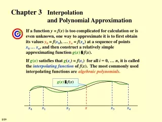
Two steps for the conceptually interpolation process: • Fit an interpolation function to the data points provided. • Evaluate that interpolating function at a target point x.
Disadvantages for the above two-stage method: • Less efficient. • More susceptible to round-off error. Many practical schemes start at a nearby point f(xi), and then add a sequence of (hopefully) decreasing corrections, as information from other nearby f(xi)’s is incorporated.
The order of the interpolation: The number of points – 1 used in an interpolation scheme. Increasing the order does not necessarily increase the accuracy, especially in polynomial interpolation. adding points close to the desired point usually does help, but a finer mesh implies a larger table of values, which is not always available.
Searching an Ordered Table: • Given an array xj, j = 0, …, N – 1, with the monotonically increasing or monotonically decreasing , and given an integer M <= N, and a number , find an interger j10such that x is among the xj10, …, xj10+M-1. x should lies between xm and xm+1, where • Bisection is the best way to solve the problem.
Search with Correlated Values: Not good to do a full bisection when interpolation routines are called multiply times. Hunt method starts with a random position in the table. It first “hunts,” either up or down, in increments of 1, then 2, then 4, etc., until the desired value is bracketed. It then bisects in the bracketed interval.
hunt algorithm Function hunt( double x) { //check xx[] is monotonic increasing or decreasing //define jl as start point, ju as end point, inc as increment value //move to right side if true. if(x >= xx[jl]) { for(;;) { //update ju equal to jl plus increment value //if ju >= n-1 or x < xx[ju], break; //else update jlequal to ju, and increment * 2 } } else { for(;;) { //update jlequal to jlminus increment value //if jl <= 0 or x >= xx[jl], break; //else update juequal to jl, and increment * 2 } } bisection algorithm; }
Cubic Spline Interpolation • We start from a set of points [xi, yi] for i = 0, 1, …, n for the function y = f(x). The cubic spine interpolation is a piecewise continuous curve, passing through each of the values in the table. • Spline of degree k = 3 • The domain of s is an interval [a, b] • S, S’, S’’ are all continuous functions on [a, b]
S0(x) , x [x0, x1] S(x) = S1(x) , x [x1, x2] … Sn-1(x) , x [xn-1, xn] Si(x) is a cubic polynomial that will be used on the subinterval [xi, xi+1].
There is a separate cubic polynomial for each interval [xj-1, xj], each with its own coefficients: • S(x) = sj(x) = ajx3 + bjx2 + cjx + djx (xj—1, xj), j = 1,2,…n • 4 coefficients with n subintervals = 4n equations • There are 4n-2 conditions • Interpolation conditions • Continuity conditions
Set one or both of y0’’ and yN-1’’ equal to 0. S’’(x0) = 0, S’’(xn) = 0. Set either of y0’’ andyN-1’’ to values calculate from first derivative function so as to make the first derivative of the interpolating function have a specified value on either or both boundaries.
The gold of cubic spline interpolation: Smooth in the first derivative Continuous in the second derivative. Thus means : s(xj – 0) = s(xj + 0) s’(xj – 0) = s’(xj + 0) j = 1,2, …, n - 1 s’’(xj – 0) = s(xj + 0)
Assuming s’’(xi) = Mi (i = 0, 1, 2, …, n). Because s(x) is third degree polynomial between xi and xi+1, so s’’(x)is first degree polynomial in [xi , xi+1], which is:
Taylor series: So, we can get : Let x = xi + 1