Download
1 / 48
480 likes | 677 Vues
Network Layer: Routing. UIUC CS438: Communication Networks Summer 2014 Fred Douglas Slides: Fred, Caesar&many others (edited ). 5. 3. 5. 2. 2. 1. 3. 1. 2. 1. C. D. B. A. E. F. Routing Protocols . Routing protocols implement the core function of a network

E N D
Network Layer: Routing UIUC CS438: Communication Networks Summer 2014 Fred Douglas Slides: Fred, Caesar&manyothers (edited)
5 3 5 2 2 1 3 1 2 1 C D B A E F Routing Protocols • Routing protocols implement the core function of a network • Establish paths between nodes • Part of the network’s “control plane” • Network modeled as a graph • Routers are graph vertices • Links are edges • Edges have an associated “cost” • e.g., distance, loss • Goal: compute a “good” path from source to destination • “good” usually means the shortest (least cost) path
Addressing (for now) • Assume each host has a unique ID (address) • No particular structure to those IDs • Later in course will talk about real IP addressing
Dijkstra’s Shortest-path Algorithm • Assumption: we are a central entity that sees the entire network • Input: a graph, with costs assigned to edges • (Theoryland assumption: non-negative costs) • Goal: for a single node, compute that node’s cheapest paths to all other nodes
Dijkstra’s Intuition • Among our neighbors, the direct link is the shortest path to at least one of them • This holds inductively if we compute best paths to be a connected group, and consider the group to be a single entity • Maintain two groups: • The “already know shortest path” core • The “frontier”: the core’s neighbors • One by one, move a frontier node to the core
1 1 1 4 1 2 4 1 3 3 3 2 2 2 3 2 3 1 2 4 3 3 3 1 5 2 3 1 1 1 S 7 8
c(i,j): link cost from node ito j; cost is infinite if not direct neighbors; ≥ 0 D(v):total cost of the current least cost path from source to destination v p(v):v’s predecessor along path from source to v S: set of nodes whose least cost path definitively known D C A E B F 5 3 5 2 2 1 3 1 2 1 (BEGIN: for offline studying) Notation Source
Dijkstra’s Algorithm • c(i,j): link cost from node i to j • D(v): current cost source v • p(v): v’s predecessor along path from source to v • S: set of nodes whose least cost path definitively known 1 Initialization: 2 S = {A}; 3 for all nodes v 4 if v adjacent to A 5 then D(v) = c(A,v); 6 else D(v) = ; 7 8 Loop 9 find w not in S such that D(w) is a minimum; 10 add w to S; 11 update D(v) for all v adjacent to w and not in S: 12 if D(w) + c(w,v) < D(v) then // w gives us a shorter path to v than we’ve found so far 13 D(v) = D(w) + c(w,v); p(v) = w; 14 until all nodes in S;
D C A E B F 5 3 5 2 2 1 3 1 2 1 Example: Dijkstra’s Algorithm D(B),p(B) 2,A D(D),p(D) 1,A D(C),p(C) 5,A D(E),p(E) Step 0 1 2 3 4 5 set S A D(F),p(F) 1 Initialization: 2 S = {A}; 3 for all nodes v 4 if v adjacent to A 5 then D(v) = c(A,v); 6 else D(v) = ; …
… • 8 Loop • 9 find w not in Ss.t. D(w) is a minimum; • 10 add w to S; • update D(v) for all v adjacent • to w and not in S: • If D(w) + c(w,v) < D(v) then • D(v) = D(w) + c(w,v); p(v) = w; • 14 until all nodes in S; D C A E B F 5 3 5 2 2 1 3 1 2 1 Example: Dijkstra’s Algorithm D(B),p(B) 2,A D(D),p(D) 1,A D(C),p(C) 5,A D(E),p(E) Step 0 1 2 3 4 5 set S A D(F),p(F)
… • 8 Loop • 9 find w not in Ss.t. D(w) is a minimum; • 10 add w to S; • update D(v) for all v adjacent • to w and not in S: • If D(w) + c(w,v) < D(v) then • D(v) = D(w) + c(w,v); p(v) = w; • 14 until all nodes in S; C D E A B F Example: Dijkstra’s Algorithm D(B),p(B) 2,A D(D),p(D) 1,A D(C),p(C) 5,A D(E),p(E) Step 0 1 2 3 4 5 set S A AD D(F),p(F) 5 3 5 2 2 1 3 1 2 1
… • 8 Loop • 9 find w not in Ss.t. D(w) is a minimum; • 10 add w to S; • update D(v) for all v adjacent • to w and not in S: • If D(w) + c(w,v) < D(v) then • D(v) = D(w) + c(w,v); p(v) = w; • 14 until all nodes in S; C D E A B F Example: Dijkstra’s Algorithm D(B),p(B) 2,A D(D),p(D) 1,A D(C),p(C) 5,A 4,D D(E),p(E) 2,D Step 0 1 2 3 4 5 set S A AD D(F),p(F) 5 3 5 2 2 1 3 1 2 1
… • 8 Loop • 9 find w not in Ss.t. D(w) is a minimum; • 10 add w to S; • update D(v) for all v adjacent • to w and not in S: • If D(w) + c(w,v) < D(v) then • D(v) = D(w) + c(w,v); p(v) = w; • 14 until all nodes in S; C D E A B F Example: Dijkstra’s Algorithm D(B),p(B) 2,A D(D),p(D) 1,A D(C),p(C) 5,A 4,D 3,E D(E),p(E) 2,D Step 0 1 2 3 4 5 set S A AD ADE D(F),p(F) 4,E 5 3 5 2 2 1 3 1 2 1
… • 8 Loop • 9 find w not in Ss.t. D(w) is a minimum; • 10 add w to S; • update D(v) for all v adjacent • to w and not in S: • If D(w) + c(w,v) < D(v) then • D(v) = D(w) + c(w,v); p(v) = w; • 14 until all nodes in S; C D E A B F Example: Dijkstra’s Algorithm D(B),p(B) 2,A D(D),p(D) 1,A D(C),p(C) 5,A 4,D 3,E D(E),p(E) 2,D Step 0 1 2 3 4 5 set S A AD ADE ADEB D(F),p(F) 4,E 5 3 5 2 2 1 3 1 2 1
… • 8 Loop • 9 find w not in Ss.t. D(w) is a minimum; • 10 add w to S; • update D(v) for all v adjacent • to w and not in S: • If D(w) + c(w,v) < D(v) then • D(v) = D(w) + c(w,v); p(v) = w; • 14 until all nodes in S; C D E A B F Example: Dijkstra’s Algorithm D(B),p(B) 2,A D(D),p(D) 1,A D(C),p(C) 5,A 4,D 3,E D(E),p(E) 2,D Step 0 1 2 3 4 5 set S A AD ADE ADEB ADEBC D(F),p(F) 4,E 5 3 5 2 2 1 3 1 2 1
… • 8 Loop • 9 find w not in Ss.t. D(w) is a minimum; • 10 add w to S; • update D(v) for all v adjacent • to w and not in S: • If D(w) + c(w,v) < D(v) then • D(v) = D(w) + c(w,v); p(v) = w; • 14 until all nodes in S; C D E A B F 5 3 5 2 2 1 3 1 2 1 Example: Dijkstra’s Algorithm D(B),p(B) 2,A D(D),p(D) 1,A D(C),p(C) 5,A 4,D 3,E D(E),p(E) 2,D Step 0 1 2 3 4 5 set S A AD ADE ADEB ADEBC ADEBCF D(F),p(F) 4,E
(END: for offline studying) C D E A B F 5 3 5 2 2 1 3 1 2 1 Example: Dijkstra’s Algorithm D(B),p(B) 2,A D(D),p(D) 1,A D(C),p(C) 5,A 4,D 3,E D(E),p(E) 2,D Step 0 1 2 3 4 5 set S A AD ADE ADEB ADEBC ADEBCF D(F),p(F) 4,E To determine path A C (say), work backward from C via p(v)
Link State Intuition • A central view of the entire network lets you run Dijkstra’s algorithm… • So give everyone a central view! • Propagate information on the state of the links that you can directly see • Whether they exist • How much they cost • Run Dijkstra’s algorithm when your view of the topology changes
Link state: update propagation Each node maintains a “topology database” F tells all routers: there is a link between F and E [B,D] [D,F] [E,F] [C,E] [C,A] [C,B] [A,B] [D,E] [C,E] [D,F] [A,B] [C,B] [C,A] [D,E] [B,D] [E,F] [B,D] [D,E] [D,F] [C,B] [C,A] [A,B] [C,E] [E,F] [C,B] [C,A] [C,E] [B,D] [A,B] [E,F] [D,F] [D,E] [C,E] [C,B] [A,B] [D,F] [E,F] [B,D] [D,E] [C,A] [E,F] [D,F] [C,A] [C,E] [C,B] [B,D] [D,E] [A,B] [E,F] [B,D] [D,F] [A,B] [C,A] [D,E] [C,B] [C,E] [D,F] [C,B] [C,A] [D,E] [B,D] [A,B] [C,E] [E,F] [A,B] [D,F] [C,A] [C,E] [E,F] [D,E] [B,D] [C,B] [D,F] [C,A] [E,F] [A,B] [C,E] [C,B] [B,D] [D,E] B D A F C E • How to prevent update loops: (seq numbers) • How to bring up new node: (load TDB from neighbor)
Link state: route computation B D A F C E • Each router computes shortest path tree, rooted at that router • Determines next-hop to each dest, publish to forwarding table • Operators can assign link costs to control path selection
D C A E B F 5 3 5 2 2 1 3 1 2 1 Forwarding table: the goal • Running Dijkstra at node A gives the shortest path from A to all destinations • We then construct the forwarding table
Issue #1: Scalability • How many messages needed to flood link state messages? • O(N x E), where N is #nodes; E is #edges in graph • Processing complexity for Dijkstra’s algorithm? • O(N2), because we check all nodes w not in S at each iteration and we have O(N) iterations • more efficient implementations: O(N log(N)) • (heap) • How many entries in the LS topology database? • O(E) • How many entries in the forwarding table? • O(N)
D B O H I M E A C G J P In regular link-state, routers maintain map of entire topology Solution #1: Hierarchical routing D B O H I M E A C G J P
O H I M A Routers summarize paths across areas as “virtual links” G J P Aggregate groups of routers into “areas” “Border routers” generate “summary LSPs” to reach other border routers Solution #1: Hierarchical routing D B O H I M E A C G J P
Solution #2: Fewer Nodes! • Problem: Scaling problems at internet scale • Solution: Just don’t scale that far • Another level of hierarchy: autonomous systems • One company’s network = 1 AS • Don’t even look inside other ASes. Just find a path at the AS level: the graph where 1 node = 1 AS • Much more detail a few lectures later
Distance Vector Intuition • Think in terms of one destination at a time. • Implementation reality: the “vector” is because we actually do all of the destinations in parallel • Advertise your paths. • Use the best path you currently know of. • Send the advertisements when your best path cost changes (for better or worse) I have a cost 6 path to A I have a cost 4 path to A 2 3 A 4 B C D
Distance Vector Algorithm (for offline studying) 1 Initialization: 2 for allneighbors V do 3 ifV adjacent to A 4 D(A, V) = c(A,V); else D(A, V) = ∞; send D(A, Y) to all neighbors loop: 8 wait (until A sees a link cost change to neighbor V /* case 1 */ 9 or until A receives update from neighbor V) /* case 2 */ 10 if (c(A,V) changes by ±d) /* case 1 */ 11 for all destinations Y that go through Vdo 12 DV(A,Y) = DV(A,Y) ± d 13 else if (update D(V, Y) received from V) /* case 2 */ /* shortest path from V to some Y has changed */ 14 DV(A,Y) = DV(A,V) + D(V, Y); /* may also change D(A,Y) */ 15 if (there is a new minimum for destination Y) 16 send D(A, Y) to all neighbors 17 forever • c(i,j): link cost from node i to j • DZ(A,V): cost from A to V via Z • D(A,V):cost of A’s best path to V
Distance Vector Example I have a cost 6 path to A I have a cost 4 path to A 2 3 A 4 B C D 1 1 I have a cost 7 path to A I have a cost 5 path to A E F G 1 1 I have a cost 6 path to A
Count-to-Infinity Problem 1 A B 14 1 C
Count-to-Infinity Problem 1 A B 14 1 C
Count-to-Infinity Problem A B 14 1 C
Count-to-Infinity Problem A B ~ 14 1 C
Count-to-Infinity Problem A B ~ 14 1 C
Count-to-Infinity Problem A B ~ 3 14 1 C
Count-to-Infinity Problem A B ~ 3 14 1 C
Count-to-Infinity Problem A B ~ 3 14 1 C 4
Count-to-Infinity Problem A B ~ 3 14 1 C 4
Count-to-Infinity Problem A B ~ 3 5 14 1 C 4 (we are not going to go through the whole process )
Count-to-infinity Solutions • Let ∞ = 16 • (This is real: Routing Information Protocol) • “Poison reverse”: advertise a distance of “infinity” back to the neighbor whose path you use • Just specify the path you’re talking about…
Will Poison-Reverse Completely Solve the Count-to-Infinity Problem? (destination is D) D 100 1 ∞ 4 B 4 100 ∞ 1 100 1 1 1 6 3 ∞ ∞ 2 2 ∞ 5 A C 1 (we are not going to go through the whole process )
Link State vs Distance Vector • Conclusion: link state is just better! • Scalability • Convergence time • However, link state assumes all nodes are “working together” under the same entity… • In the real world: • RIP (distance vector) came first • OSPF, IS-IS (link state) are today’s choice
Path Vector Intuition • In your DV ads, specify the path • We can • include the total cost (like above) • just let the # of hops in the path be the cost • How does it solve count-to-infinity? • Knowing if you are already part of the path your neighbor is offering Path to A: CBA, cost 6 Path to A: BA, cost 4 2 3 A 4 B C D
Count-to-infinity revisited: path vector (destination is D) D 1 100 B BD, cost 100 BD, cost 100 BD, cost 1 BD, cost 1 1 1 ACBD, cost 102 ACBD, cost 3 CABD, cost 102 CABD, cost 3 1 A C ABD, cost 2 CBD, cost 2 ABD, cost 101 CBD, cost 101 Converged!
Routing Summary • Goal: compute optimal paths • In real world terms: establish forwarding table • Link State: learn exactly what the network looks like, run a centralized algorithm • Distance/Path Vector: pass around news of usable paths to various destinations