Download
1 / 44
440 likes | 543 Vues
Preliminary results and uncertainties of scattering measurements for SORTIE. Michael Twardowski 1 , Scott Freeman, Jim Sullivan, Ron Zaneveld, Chuck Trees, and the SORTIE Team 1 WET Labs, Inc., Narragansett, RI mtwardo@wetlabs2.com. SORTIE IOP Objectives.

E N D
Preliminary results and uncertainties of scattering measurements for SORTIE Michael Twardowski1, Scott Freeman, Jim Sullivan, Ron Zaneveld, Chuck Trees, and the SORTIE Team 1WET Labs, Inc., Narragansett, RI mtwardo@wetlabs2.com
SORTIE IOP Objectives • Use IOPs in radiative transfer models to help constrain uncertainties for radiometric measurements • Map horizontal-vertical spatial variability in optical properties around station • Evaluate and refine IOP measurement protocols • Evaluate and refine IOP uncertainties
MASCOT package MASCOT: VSF b(10:10:170 deg; 650 nm) ECOVSF: VSF b(100, 125, 150 deg; 650 nm) ECOBB3: VSF b(117 deg; 470, 532, 650 nm) AUV-B: total scattering (650 nm) AC9: a and c (9l)
Dolphin package ACS, AC9, ECO BB3, ECO BB2C, SBE49 CTD, DH4 data handler, and Notus gearfinder pinger
Estimated error Spatial Variability:cpg(532) trace during tow
Spatial Variability:Hyperspectral a and c during tow MOBY site
Mamala Bay MOBY site Spatial Variability:Vertical profiles of cpg532
VSF calibration protocol Relationship between raw VSF counts (F) and b 2 unknowns for each q: SF and e b(q) = [F(q) – DO(q)] * SF(q) * exp [ L * (bp * e + at) ] • q: angle • DO: dark offset • SF: scaling factor (relative gain) • L: pathlength (0.2 m) • : fraction of bp not reaching detector bp: particulate scattering at: total absorption pathlength attenuation term
[F(q) – DO(q)] = bp * [P(q)/ SF(q)] * exp [ - L * (bp * e + at ] VSF calibration protocol b(q) = [F(q) – DO(q)] * SF(q) * exp [ L * (bp * e + at) ] Now there are 3 unknowns for each q: P, SF and e Since there is no b “standard” for vicarious calibration, introduce particle standard with known phase function, P(q). Solve for bp: Inverting the above to solve for [F(q) – DO(q)], we obtain: bp = [F(q) – DO(q)] * [SF(q) / P(q)] * exp [ L * (bp * e + at) ]
Important Point #1 For VSF measurements, dark offsets should always be measured in-situ
[F(q) – DO(q)] = bp * [P(q)/SF(q)] * exp [ - L * (bp * e + at ] 12/15/06 MASCOT VSF calibrations Arizona Road Dust • If we assume apg650~0, we can solve for (P/SF) and e with a nonlinear fit to the empirical data for each channel • *but in practice there are relatively large error bars with this method
[F(q) – DO(q)] = bp * [P(q)/SF(q)] * exp [ - L * (bp * e + at ] ( ) MASCOT VSF calibrations Arizona Road Dust • All channels normalized to area • But we know something else: • e should be approximately constant for each detector • e = 0.56 Detector field-of-view unimportant
[F(q) – DO(q)] = bp * [P(q)/SF(q)] * exp [ - L * (bp * e + at ] MASCOT VSF calibrations Now we can solve for (P/SF) for each angle (P/SF) Microspherical beads
MASCOT VSF calibrations Phase function for 1.992±0.025 um beads
MASCOT VSF calibrations Weighting functions for MASCOT angles
MASCOT VSF calibrations Phase function values for MASCOT angles P(q)
= SF(q) theoretical P empirical P/SF MASCOT VSF calibrations Now all calibration parameters are solved
MASCOT VSF calibrations Calibrated VSFs from the AZRD exp’t Concurrent ECO-VSF measurements
10 m binned VSFs from Hawaii MASCOT ECO-VSF
b(q) profiles from Hawaii MASCOT ECO-VSF
b(q) profiles from Hawaii MASCOT with ECO-VSF overlay bsw(150°,650 nm)
Pure water scattering Twardowski et al. 2007
Important Point #2 In clear water, accurate pure seawater VSF values are critical for deriving particulate VSF values
Agreement with theoretical modeling Fournier-Forand phase functions
ECO-BB3 comparisons 3 different devices
MVSM (Ukrainian device at NRL) ECOVSF MASCOT More VSF comparisons NY Bight: May 2007
More VSF comparisons NY Bight: May 2007
Backscattering analysis: from Hawaii and NY Bight apparent underestimation of bb by ECOVSF by few percent
Backscattering analysis: from Hawaii and NY Bight ECOVSF 3rd order polynomial (polyfit) method for obtaining bb ~4% difference now ~8% underestimation of bb by polyfit method MASCOT polyfit MASCOT fully integrated bb ECOVSF polyfit
Important Point #3 Currently recommended “polyfit” method appears to underestimate bbp by a few percent This is because the polyfit extrapolation to 90 degrees from the 100-125-150 degree measurements is not quite steep enough.
Backscattering analysis So why do we use it? Ocean Optics 2000 Monaco
Analysis of shape of VSF in backward direction 150° vs 125° for 9 different coastal US sites Sullivan et al. 2005: 532 nm ECO-VSF
Analysis of shape of VSF in backward direction Adding 657 nm ECO-VSF NY Bight data
Analysis of shape of VSF in backward direction Adding 650 nm MASCOT NY Bight data
Analysis of shape of VSF in backward direction 100° vs 125° for 9 different coastal US sites Sullivan et al. 2005: 532 nm ECO-VSF
Analysis of shape of VSF in backward direction Adding 657 nm ECO-VSF NY Bight data
Analysis of shape of VSF in backward direction Adding 650 nm MASCOT NY Bight data
Lowest prediction errors in estimating backscattering coefficient [ Consistent with Oishi 1990; Boss and Pegau 2001 MASCOT % variation inbbp normalized data (2pb(q)/bbp)
Important Point #4 a) bp(110-120) is best range to pick a single angle measurement for estimating bbp b) using 1 or a few angles to estimate bbp has merit c) No obvious spectral variability in VSF shape was observed
VSF Uncertainties Table 3. Parameters from scattering measurements in the South Pacific central gyre. All values expressed in 10-4. Twardowski, M.S., H. Claustre, S.A. Freeman, D. Stramski, and Y. Hout. 2007. Optical backscattering properties of the “clearest” natural waters. Biogeosciences, 4, 1041–1058. • Detailed Methodology • Detailed uncertainties analysis • Dark offsets measured in-situ for the first time • New values for pure seawater scattering recommended ai.e., random electronic error bcomputed over 1-m depth bins; see text cpure water scattering computed from Buiteveld et al. (1994) at 20°C; [1 + 0.3(35)/37] adjustment for dissolved salts applied after Morel (1974)
Summary 1. For VSF measurements, dark offsets should be measured IN SITU 2. In clear ocean water, accurate pure seawater VSF values are critical for deriving particulate VSF values 3. More work may be needed to refine method of estimating bbp from 3-angle measurements 4. Shape of VSF in the backward direction is remarkably consistent i. bp(110°-120°) is the best range for picking a single angle measurement for estimating bbp • ii. Using 1 or a few angles to estimate bbp has merit • iii. No obvious spectral variability in VSF shape was • observed