Download
1 / 52
550 likes | 681 Vues
Precipitation. Introduction. Moisture in the Atmosphere. Evaporation Water changes from liquid to vapor Evaporation and precipitation controlled by: Air temperature Moisture content of the atmosphere The relative humidity is a measure of the amount of water in the air.

E N D
Precipitation Introduction
Moisture in the Atmosphere • Evaporation • Water changes from liquid to vapor • Evaporation and precipitation controlled by: • Air temperature • Moisture content of the atmosphere • The relative humidity is a measure of the amount of water in the air
Moisture in the Atmosphere • Precipitation is formed from water vapor • As air cools its capacity to hold water decreases • Saturated (100% relative humidity) • Saturation at 70 oF vs. 32 oF • Air can hold 4 times more water at 70 oF • Cooling effect can cause moist unsaturated air to become saturated (dew point) • Cooling beyond 100 % saturation causes water vapor to condense and change to liquid or solid water. • Water droplets on cold glass / dew on grass/hail
The relationship between water content of air at saturation and air temperature
Precipitation Occurs when three conditions are met: • Atmosphere is saturated • Atmosphere becomes saturated when the air mass is cooled usually by lifting. • Air mass lifting caused by: • Frontal systems (warm moist air meets colder heavier air). • Orographic effects (induced by mountains) • Convection (air expands when heated by solar energy and becomes lighter than the air around it.
Precipitation • Small particles are present • Dust, ocean salt, smoke • Drops reach a size that causes them to fall toward Earth. • May collect additional condensed vapor • May evaporate
Frontal Systems • Cold fronts • High intensity / short duration / narrow zone • Typical in the spring and fall • Warm fronts • Gentle rainfall / long term / widespread • Typical in the winter • Orographicprecipitation • Increasing rainfall with increasing elevation • Convective precipitation • High intensity / short duration / limited area • Earth surface and air close to surface heated lifted • Typical summer thunderstorm
Typical in the winter Typical in the spring and fall Typical in the summer
Cold front producing a high intensity rainfall event. Cold air coming from the left colliding with warm air on the right.
Precipitation Measurement, Estimation and Probability
Precipitation Data • Necessary for most land use plans • Municipal / industrial / agricultural / forestry / flood prevention / recreation • Data collection by State and Federal agencies • Much of the data is now on-line via the internet • Precipitation records report amounts • Yearly / monthly / daily / hourly
Rainfall • Large variation depending on • Location and time of year • Some deserts get 0 rain • Cherrapunji, India has gotten 1000 in./yr (83 ft) • Combined orographic effects and monsoons • Units of measurement depth (in. / mm / etc.) • Can get volume easily by multiplying by area • Accuracy of measurement 0.01 in. • Mis-leading since no two rain gages will ever record the same amount of rain even if they are side by side!
Rainfall • Data widely available. • Typically two types of rain gauges • Non-recording • Low cost / maintenance free • Accuracy = 0.1 in. • Recording • NEXRAD
Recording Rain Gages • Weighing bucket type • Good for large rainfall events • Can’t accurately measure (weigh) small rainfall events • Tipping bucket type • Good for small rainfall events • Can’t keep up during heavy rainfall events. • Each tip = 0.01”
Snow-Pack Measurement • 80 to 90% of annual precipitation is snow in some areas • High elevation snow country is often forested • 75% of the water supply in western U.S. is from forests • Water equivalent (depth after melting) • For fresh snow 10 inches deep: • 5% to 20% = 0.5” to 2.0” of water • For snow in late summer up to 60%
Rainfall Measurement • Standard rain gages are point samples only • Generally a high degree of variation in any rainfall • Rain gages are usually cylindrical with circular top • Therefore least subjected to edge effect errors • Mounted vertically • Height of 2 m (about 6 ft) • 2:1 obstruction rule • If top of object is 30 ft above gage • Place gage 60 ft away • Eliminates obstructions that may affect rainfall capture
What we want: Total rainfall amount volume = depth x area Rainfall intensity in./hr or mm / hr Rainfall distribution Over time Over space What we have: Point measurements at a few locations Must extrapolate over the entire watershed Measurement of Precipitation
Rainfall on a Watershed Scale • 3 common methods for estimating average rainfall. • Arithmetic Mean • Thiesson polygon method • Isohyetal method
Arithmetic mean method Assumes uniform rainfall distribution Very seldom occurs Easiest to use but least accurate Thiessen polygon method Assumes linear variation Use when gages are not uniformly distributed Can use gages outside of watershed Isohyetal method Theoretically the most accurate Most time consuming method Can use gages outside of the watershed Calculating Average Precipitation Over an Area
Measured Rainfall at Six Rainfall Gages Watershed boundary P6 = 1.81” P2 = 2.15” P4 = 2.26” P1 = 1.62” P5 = 2.18” P3 = 1.80”
Pavg = [ Wi x Pi ] / Wi All gages given equal weight Weight = 1 Pavg = (1.82 + 2.15 + 2.26 + 2.18 + 1.62 + 1.8) / 6 Pavg = 1.97 in. Arithmetic Mean Method
First: Draw straight dashed lines between each rainfall gage Second: Draw solid perpendicular bisectors to these lines so that watershed area associated with each gage is enclosed by bisector lines These enclosed areas are known as Thiessen Polygons The area within each polygon is closer to the rain gage enclosed than any other rain gage. The rainfall measured in the polygon is assumed to be representative of the rainfall in the entire polygon Thiessen Polygon Method
Third: Determine the area of each polygon The rain gage weight is the area of the polygon it is located in Fourth: Calculate the average rainfall using: Pavg = [ Wi x Pi ] / Wi Thiessen Polygon Method
Step #1: Dashed Lines Between Each Rain Gage Watershed boundary P6 = 1.81” P2 = 2.15” P4 = 2.26” P1 = 1.62” P5 = 2.18” P3 = 1.80”
Step #2: Draw the Perpendicular Bisector Lines Watershed boundary
Step #3: Determine the Area of Each Polygon Watershed boundary A4= 269 ac A6= 65 ac A2= 150 ac A1= 56 ac A5= 216 ac A3= 136 ac
Pavg = [ Wi x Pi ] / Wi Pavg = [(65x1.81)+(150x2.15)+(269x2.26)+ (216x2.18)+(56x1.62)+(136x1.8)] / [65+150+269+ 216+56+136] Pavg = 2.08 in. Step #4: Calculate the Average Rainfall
Mean Annual Rainfall in inches with the longitude parallels 98o and 100o also shown
Point Precipitation Patterns • Often want to predict rain in the future rather than use historical rainfall • Rainfall Depth-Duration and Frequency • Rainfall Intensity-Duration and Frequency • TP 40 and similar documents provide this information.
Precipitation Data • When planning/designing we need to know three things. • What is the depth or intensity of the rainfall we are designing for? • What is the length of time (duration) of that rainfall? • How often will rainfall of that depth and duration return (what is its frequency?)
Return Period and Probability • T-year event – an event of such magnitude that over a long period of time, the average time between events having a magnitude greater than the T-year event is T years. • The expected number of occurrences of a T-year event in an N-year period is N/T. • On average we expect a T-year event to occur once in T-years.
Rainfall and Frequency • The 25-yr, 24-hr rainfall for Houston is 10 in. (25 cm) • The depth is 10 inches, the duration is 24 hours and the frequency is 25 years. • The frequency is also known as the return period. • This means that on average a 10 in. rainfall event will occur four times in 100 yrs . • It does not mean that a 10 in. rainfall event will happen exactly every 25 years and it does not mean that there will be exactly 4, 10 in. rainfall events in 100 yrs. • The probability of a T-yr event in any given year is a 1/T • A 25 year event has a 4% chance of occurring in a single year (1/25 * 100). • Likewise a 10 yr event = 10% chance [(1/10)*100] • Likewise a 50 yr event = 2% chance [(1/50)*100]
Depth (OR Intensity) -Duration and Frequency Curves • DDF or IDF curves have been developed for many cities and locations around the U.S. • When using an IDF curve rainfall depth (in) is found by multiplying the intensity (in/hr) by the duration (hr).
Rainfall / Flood Return Frequency and Duration • Return frequency used in engineering designs: • Depends on economic value • Rural roads (not much traffic) 5 to 10 year return • Interstate highways 50 to 100 year return period • Design duration depends on size of watershed • Small to medium watersheds (1 to 100 mi2) • Duration of 5 minutes to 24 hours • Large watersheds (over 100 mi2) up to 1 mo. duration • River basin studies up to 1 yr may be needed
10 yr 24 hour DDF http://www.srh.noaa.gov/lub/wx/precip_freq/precip_index.htm
Publications of DDF • TP-40 • Contains DDF data for the U.S. for durations of 30 min. to 24 hr and frequencies from 1 to 100 years. • HYDRO-35 • Gives DDF for Eastern US for durations of 5 to 60 minutes and frequencies to 100 years. • NOAA Atlases • For use in western U.S.
Rainfall Time Distribution • Ultimately we are building up to developing runoff hydrographs (runoff depth vs. time). • In order to do so we need not only depth, duration and frequency of a storm but also distribution of rainfall within its duration. • Plot of time distribution of rainfall intensity is known as the rainfall hyetograph.
AGSM 335 • Homework #2
Rainfall Hyetograph • Two most common ways to design: • Adopt a historical storm that has occurred in the vicinity and has caused damage OR • Develop a synthetic design storm
Historical Rainfall Approach • Advantages • Readily identified and explained to engineers and the public. • Disadvantages • Unknown frequency of occurrence. • Difficulty in associating a return period with a particular rainfall time-intensity pattern. • These difficulties have lead to the development of synthetic storms.
Synthetic storms • Advantages • Consistent basis for design • Disadvantages • Very remote possibility of ever happening exactly as specified. • Represent reasonable approximations to actual storm patterns that might be expected for a given return period.
Methods for developing synthetic storms • Balanced Storm Methods • DDF Rainfall Pattern • SCS Rainfall Pattern
SCS Rainfall Pattern • Uses several dimensionless rainfall temporal patterns called Type Curves
Applicable Regions for SCS Type Curves • Divides the U.S. into 4 rainfall patterns Type I Alaska, S. California and Hawaii • Type IA Pacific Northwest (least intense for short durations). • Type II Mostly Non-Coastal U.S. (most intense) • Type III E. Coast and Gulf Coast
SCS Method • Based on 24-hr storm of desired frequency. • Rainfall is proportioned through the 24-hr period using the appropriate curve in the form of percentage mass curves. .
Method for creating a rainfall Hyetograph Using the SCS Type curves • Determine the storm Type for the area of interest. • Determine the duration and frequency of the storm. • Look up the 24 hr rainfall (P24) for the frequency you choose (Appendix C, Page 445). • For a 24 hr storm, multiply each of the values in Table 3.4 (Handout on webpage) by the P24. Result is the 24 hr rainfall pattern for the frequency you chose. • Calculate the Incremental P depths. • For durations less than 24 hours center the storm on the steepest part of the type curves is used (generally centered somewhere around 12 hrs). • Graph the incremental P vs. Time.