Download
1 / 27
280 likes | 549 Vues
The EM algorithm, and Fisher vector image representation. Jakob Verbeek December 17, 2010 Course website: http://lear.inrialpes.fr/~verbeek/MLCR.10.11.php. Plan for the course. Session 1, October 1 2010 Cordelia Schmid: Introduction Jakob Verbeek: Introduction Machine Learning

E N D
The EM algorithm, and Fisher vector image representation Jakob Verbeek December 17, 2010 Course website: http://lear.inrialpes.fr/~verbeek/MLCR.10.11.php
Plan for the course • Session 1, October 1 2010 • Cordelia Schmid: Introduction • Jakob Verbeek: Introduction Machine Learning • Session 2, December 3 2010 • Jakob Verbeek: Clustering with k-means, mixture of Gaussians • Cordelia Schmid: Local invariant features • Student presentation 1: Scale and affine invariant interest point detectors, Mikolajczyk, Schmid, IJCV 2004. • Session 3, December 10 2010 • Cordelia Schmid: Instance-level recognition: efficient search • Student presentation 2: Scalable Recognition with a Vocabulary Tree, Nister and Stewenius, CVPR 2006.
Plan for the course • Session 4, December 17 2010 • Jakob Verbeek: The EM algorithm, and Fisher vector image representation • Cordelia Schmid: Bag-of-features models for category-level classification • Student presentation 2: Beyond bags of features: spatial pyramid matching for recognizing natural scene categories, Lazebnik, Schmid and Ponce, CVPR 2006. • Session 5, January 7 2011 • Jakob Verbeek: Classification 1: generative and non-parameteric methods • Student presentation 4: Large-Scale Image Retrieval with Compressed Fisher Vectors, Perronnin, Liu, Sanchez and Poirier, CVPR 2010. • Cordelia Schmid: Category level localization: Sliding window and shape model • Student presentation 5: Object Detection with Discriminatively Trained Part Based Models, Felzenszwalb, Girshick, McAllester and Ramanan, PAMI 2010. • Session 6, January 14 2011 • Jakob Verbeek: Classification 2: discriminative models • Student presentation 6: TagProp: Discriminative metric learning in nearest neighbor models for image auto-annotation, Guillaumin, Mensink, Verbeek and Schmid, ICCV 2009. • Student presentation 7: IM2GPS: estimating geographic information from a single image, Hays and Efros, CVPR 2008.
Clustering with k-means vs. MoG Hard assignment in k-means is not robust near border of quantization cells Soft assignment in MoG accounts for ambiguity in the assignment Both algorithms sensitive for initialization Run from several initializations Keep best result Nr of clusters need to be set Both algorithm can be generalized to other types of distances or densities Images from [Gemert et al, IEEE TPAMI, 2010]
Clustering with Gaussian mixture density Mixture density is weighted sum of Gaussians Mixing weight: importance of each cluster Density has to integrate to unity, so we require
Clustering with Gaussian mixture density Given: data set of N points xn, n=1,…,N Find mixture of Gaussians (MoG) that best explains data Parameters: mixing weights, means, covariance matrices Assume data points are drawn independently Maximize log-likelihood of data set X w.r.t. parameters As with k-means objective function has local minima Can use Expectation-Maximization (EM) algorithm Similar to the iterative k-means algorithm
Maximum likelihood estimation of MoG Use EM algorithm Initialize MoG parameters E-step: soft assign of data points to mixture components M-step: update the parameters Repeat EM steps, terminate if converged Convergence of parameters or assignments E-step: compute posterior on z given x: M-step: update parameters using the posteriors
Maximum likelihood estimation of MoG Example of several EM iterations
Bound optimization view of EM The EM algorithm is an iterative bound optimization algorithm Goal: Maximize data log-likelihood, can not be done in closed form Solution: maximize simple to optimize bound on the log-likelihood Iterations: compute bound, maximize it, repeat Bound uses two information theoretic quantities Entropy Kullback-Leibler divergence
Entropy of a distribution Entropy captures uncertainty in a distribution Maximum for uniform distribution Minimum, zero, for delta peak on single value Connection to information coding (Noiseless coding theorem, Shannon 1948) Frequent messages short code, optimal code length is (at least) -log p bits Entropy: expected code length Suppose uniform distribution over 8 outcomes: 3 bit code words Suppose distribution: 1/2,1/4, 1/8, 1/16, 1/64, 1/64, 1/64, 1/64, entropy 2 bits! Code words: 0, 10, 110, 1110, 111100, 111101,111110,111111 Codewords are “self-delimiting”: code is of length 6 and starts with 4 ones, or stops after first 0. Low entropy High entropy
Kullback-Leibler divergence Asymmetric dissimilarity between distributions Minimum, zero, if distributions are equal Maximum, infinity, if p has a zero where q is non-zero Interpretation in coding theory Sub-optimality when messages distributed according to q, but coding with codeword lengths derived from p Difference of expected code lengths Suppose distribution q: 1/2,1/4, 1/8, 1/16, 1/64, 1/64, 1/64, 1/64 Coding with uniform 3-bit code, p=uniform Expected code length using p: 3 bits Optimal expected code length, entropy H(q) = 2 bits KL divergence D(q|p) = 1 bit
EM bound on log-likelihood Define Gauss. mixture p(x) as marginal distribution of p(x,z) Posterior distribution on latent cluster assignment Let qn(zn) be arbitrary distribution over cluster assignment Bound log-likelihood by subtracting KL divergence D(q(z) || p(z|x))
Maximizing the EM bound on log-likelihood E-step: fix model parameters, update distributions qn KL divergence zero if distributions are equal Thus set qn(zn) = p(zn|xn) M-step: fix the qn, update model parameters Terms for each Gaussian decoupled from rest !
Maximizing the EM bound on log-likelihood Derive the optimal values for the mixing weights Maximize Take into account that weights sum to one, define Take derivative for mixing weight k>1
Maximizing the EM bound on log-likelihood Derive the optimal values for the MoG parameters Maximize
EM bound on log-likelihood L is bound on data log-likelihood for any distribution q Iterative coordinate ascent on F E-step optimize q, makes bound tight M-step optimize parameters
Clustering for image representation For each image that we want to classify / analyze Detect local image regions For example affine invariant interest points Describe the appearance of each region For example using the SIFT decriptor Quantization of local image descriptors using k-means or mixture of Gaussians (Soft) assign each region to clusters Count how many regions were assigned to each cluster Results in a histogram of (soft) counts How many image regions were assigned to each cluster Input to image classification method Off-line: learn k-means quantization or mixture of Gaussians from data of many images
Clustering for image representation Detect local image regions For example affine invariant interest points Describe the appearance of each region For example using the SIFT decriptor Quantization of local image descriptors using k-means or mixture of Gaussians Cluster centers / Gaussians learned off-line (Soft) assign each region to clusters Count how many regions were assigned to each cluster Results in a histogram of (soft) counts How many image regions were assigned to each cluster Input to image classification method
Fisher vector representation: motivation Feature vector quantization is computationally expensive in practice Run-time linear in N: nr. of feature vectors ~ 10^3 per image D: nr. of dimensions ~ 10^2 (SIFT) K: nr. of clusters ~ 10^3 for recognition So in total in the order of 10^8 multiplications per image to obtain a histogram of size 1000 Can we do this more efficiently ?! Yes, store more than the number of data points assigned to each cluster centre / Gaussian Reading material:“Fisher Kernels on Visual Vocabularies for Image Categorization” F. Perronnin and C. Dance, in CVPR'07 Xerox Research Centre Europe, Grenoble 20 10 5 3 8
Fisher vector image representation MoG / k-means stores nr of points per cell Need many clusters to represent distribution of descriptors in image But increases computational cost Fisher vector adds 1st & 2nd order moments More precise description of regions assigned to cluster Fewer clusters needed for same accuracy Per cluster also store: mean and variance of data in cell 20 10 20 5 5 3 8 10 8 3
Image representation using Fisher kernels General idea of Fischer vector representation Fit probabilistic model to data Use derivative of data log-likelihood as data representation, eg.for classification See [Jaakkola & Haussler. “Exploiting generative models in discriminative classifiers”, in Advances in Neural Information Processing Systems 11, 1999.] Here, we use Mixture of Gaussians to cluster the region descriptors Concatenate derivatives to obtain data representation
Image representation using Fisher kernels Extended representation of image descriptors using MoG Displacement of descriptor from center Squares of displacement from center From 1 number per descriptor per cluster, to 1+D+D2 (D = data dimension) Simplified version obtained when Using this representation for a linear classifier Diagonal covariance matrices, variance in dimensions given by vector vk For a single image region descriptor Summed over all descriptors this gives us 1: Soft count of regions assigned to cluster D: Weighted average of assigned descriptors D: Weighted variance of descriptors in all dimensions
Fisher vector image representation MoG / k-means stores nr of points per cell Need many clusters to represent distribution of descriptors in image Fischer vector adds 1st & 2nd order moments More precise description regions assigned to cluster Fewer clusters needed for same accuracy Representation (2D+1) times larger, at same computational cost Terms already calculated when computing soft-assignment Comp. cost is O(NKD), need difference between all clusters and data 20 5 8 10 3
Images from categorization task PASCAL VOC Yearly “competition” since 2005 for image classification (also object localization, segmentation, and body-part localization)
Fisher Vector: results BOV-supervised learns separate mixture model for each image class, makes that some of the visual words are class-specific MAP: assign image to class for which the corresponding MoG assigns maximum likelihood to the region descriptors Other results: based on linear classifier of the image descriptions Similar performance, using 16x fewer Gaussians Unsupervised/universal representation good
How to set the nr of clusters? Optimization criterion of k-means and MoG always improved by adding more clusters K-means: min distance to closest cluster can not increase by adding a cluster center MoG: can always add the new Gaussian with zero mixing weight, (k+1) component models contain k component models. Optimization criterion cannot be used to select # clusters Model selection by adding penalty term increasing with # clusters Minimum description length (MDL) principle Bayesian information criterion (BIC) Aikaike informaiton criterion (AIC) Cross-validation if used for another task, eg. Image categorization check performance of final system on validation set of labeled images For more details see “Pattern Recognition & Machine Learning”, by C. Bishop, 2006. In particular chapter 9, and section 3.4
How to set the nr of clusters? Bayesian model that treats parameters as missing values Prior distribution over parameters Likelihood of data given by averaging over parameter values Variational Bayesian inference for various nr of clusters Approximate data log-likelihood using the EM bound E-step: distribution q generally too complex to represent exact Use factorizing distribution q, not exact, KL divergence > 0 For models with Many parameters: fits many data sets Few parameters: won’t fit data well The “right” nr. of parameters: good fit Data sets