Download
1 / 18
180 likes | 367 Vues
Homework Solution. Initially, lump A is at 100 ºC and lump B is at 50ºC. Calculate the equilibrium temperature of the combined A+B system for the conditions (a) C V A = 2 C V B and (b) 2C V A = C V B. C V A (T f – T i A ) = -C V B (T f – T i B ) If C V A = 2 C V B , this reduces to

E N D
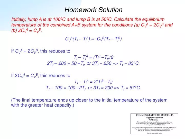
Homework Solution Initially, lump A is at 100ºC and lump B is at 50ºC. Calculate the equilibrium temperature of the combined A+B system for the conditions (a) CVA = 2CVB and (b) 2CVA = CVB. CVA(Tf – TiA) = -CVB(Tf – TiB) If CVA = 2CVB, this reduces to Tf – TiA = (TiB –Tf)/2 2Tf – 200 = 50 –Tf, or 3Tf = 250 => Tf = 83°C. If 2CVA = CVB, this reduces to Tf – TiA = 2(TiB –Tf) Tf – 100 = 100 –2Tf, or 3Tf = 200 => Tf = 67°C. (The final temperature ends up closer to the initial temperature of the system with the greater heat capacity.)
Vibrational Degrees of Freedom: Solids Simple solids like Ar(s) and metals can be treated as systems with only vibrational degrees of freedom. Statistical thermodynamics allows the apparently diverse heat capacity behaviour of solids:- …to be explained by their characteristic temperature. High-temperature-limit 0 at low T LK Nash “Elements of Statistical Thermodynamics”
Systems with Many Degrees of Freedom The ideal atomic gas has only one type of degree of freedom - translational. In order to understand realistic chemical systems, we need to be able to deal with multiple degrees of freedom. Recall that the energy of a molecule in a given molecular state, is simply the sum of the energies of each degree of freedom, translational, rotational, vibrational and electronic, viz. emolecule = etranslation + erotation + evibration + eelectronic Using our definition of the total energy of a system, we can similarly write it as a sum of components Emolecule = Etranslation + Erotation + Evibration + Eelectronic …if the degrees of freedom are independent of each other. That is, if a change in vibrational state does not cause any change in any of the other allowed energies. E.g. No Coriolis coupling between rotation and vibrations.
Heat Capacity of Diatomic Gases Once we can separate independent energies, we can also write the heat capacity as a sum of independent components CVmolecule = dE/dT|V= CVtranslation + CVrotation + CVvibration + CVelectronic Each degree of freedom has its own set of allowed energies, partition function, characteristic temperature, and heat capacity. For a diatomic gas there are 3 translations, one rotation, one vibration, and one set of electronic states. (More complex systems just have more vibrational and rotational modes.) So far we have Translation:Qtrans ~ 0K Vibration:Qvib ~ hn/kB This is the high-temperature value of the vibrational heat capacity, which occurs when T >> Qvib. Like translation, CV increases from zero below Qvib to its constant maximum value.
Non examinable: Where did the heat capacity come from? (e.g. vibrational) • Final (non-examinable) slide of lecture 3 had the following equation: • For vibrations, at high T, we can solve this with: • The definition of heat capacity gives: • So if N=1 mol, the molar heat capacity is NAkB=R
Rotations The rotational energy levels of a diatomic molecule are given by Where I is the moment of inertia of the molecule …where m1andm2 are the masses of the nuclei, and r is the bond length. The characteristic rotational temperature is given by Qrot is below 5K for all but the lightest molecules. Cvrot = nR far above Qrot. rot(H2) = 85K rot(H2O) = 40K rot(SO2) = 3K
Flash Quiz! • Calculate Qrot for the following diatomic molecules: • HD (bond length 74pm) • HF (bond length 92pm) • HI (bond length 161pm) Data: NA = 6.022×10²³ mol-1 kB = 1.38×10⁻²³ JK-1 h = 6.626×10⁻³⁴ Js p = 3.1415 MH = 1 g/mol, MD = 2 g/mol, MF = 19 g/mol, MI = 127 g/mol
Answer • Calculate Qrot for the following diatomic molecules: • HD (bond length 74pm) • HF (bond length 92pm) • HI (bond length 161pm)
Heat Capacity versus T The energy gap between ground and the first excited electron state is typically very large (i.e. elec > 104K) for diatomics and, hence, there is vanishingly small probability of there being any significant excitation at temperatures of interest. (This is not so for large molecules and solids.) A large energy gap means a large elec and, assuming that T << elec, we have CVelec 0. Putting these contributions to the heat capacity of a gas of H2 together we have something which looks as follows:-
Heat Capacity versus T The data shown below for diatomic molecules has temperature scaled by the characteristic vibrational temperature, as we did for solids, but also shows molar heat capacity scaled by R. This data focuses on vibrations only; The heat capacity increases from 5R/2 (translation + rotation) towards 7R/2 (translations + rotation + vibration) LK Nash “Elements of Statistical Thermodynamics”
Chemical Equilibrium So far we have considered changes in the equilibrium state associated with a change in energy - i.e. a gas or solid (or a liquid) whose state has been altered by heat flow or work being done. We are also interested in processes which change the numbers of various molecular components - i.e chemical reactions. Often these number changes are associated with energy changes, e.g. 2H2 + O2 = 2H2O with heat released What does this sort of process look like statistically? Consider an isomerization reaction The species A and B could, for example, stand for the ‘boat’ and ‘chair’ conformers of cyclohexane, or cis and trans conformers of 2‑butene. Thanks to the isomerization process particles have access to both A states and to B states. To start with we shall assume the molecular states of the two species resemble the follow simple ‘ladder’ of states. A⇌B
Chemical Equilibrium We return briefly to small systems. Consider the system N = 10 an E = 5 quanta. First, let’s start with ten A molecules. We already worked out that the most probable configuration is n0A = 6, n1A = 3, n2A = 1 with W = 840 microstates. Now let’s allow the isomerization reaction to occur. The most probable configuration in this case is n0A = 3, n0B = 3, n1A = 2, n1B = 1, n2B = 1 with W = 50400 microstates This is a huge increase in the number of microstates made available by accessing the energy levels of the B isomer.
Chemical Equilibrium The number of molecules of each species are obtained by adding up the occupation numbers of the two sets of molecular states. (* denotes most probable configuration.) We can define the equilibrium constant as , assuming that both A and B are ideal gases. Notice that the equilibrium configuration involves an equal number of A and B molecules. This is not surprising given that we have made them with identical states. Now we consider what happens when the energy levels of the two species are not the same.
Chemical Equilibrium In this system the ground state of B lies 1 quantum of energy below the ground state of A. This means that the overall ground state of the combined set of energy levels is 0B. The most probable configuration of this new system is n0A = 2, n0B = 6, n1A = 1, n1B = 1 with W = 2520 microstates Note that, when adding up the number of quanta, you must count 0Aas being at 1 quantum since it is 1 quantum above the overall ground state 0B. That is, 0A has the same energy as 1B. We proceed likewise for the excited states of A. The equilibrium numbers of the two species now reflect the difference in the molecules. We now find more molecules of type B than of type A, in the most probable distribution.
Chemical Equilibrium So our statistical approach to chemical equilibrium is • determine the equilibrium configuration over the combined reactant and product states, • then calculate the relative number of product and reactant molecules. CHEMICAL EQUILIBRIUM IS DETERMINED SIMPLY BY THE SYSTEM ADOPTING THE CONFIGURATION WITH THE GREATEST NUMBER OF MICROSTATES. Our next (and final) task is to put all this into a more general form. The most probable configuration is given by In this expression, n0* is the occupation number of the lowest energy state of A or B (which is e0B in the previous example). Similarly, q is the partition function considering both A and B states, and N = NA + NB is the total number of molecules in the system.
Chemical Equilibrium We can now express the equilibrium ratio of products to reactants (equal to the equilibrium constant for ideal gases) as Notice that the same ground state(which is e0B in the previous example) is used in both the numerator and denominator of this expression. Continuing with this convention, the numerator is now simply the molecular partition function for B, qB. The denominator just requires a little rearrangement:-
Chemical Equilibrium We substitute this into out equilibrium constant expression to get Chemical equilibrium, and particularly the equilibrium constant, is determined by the ratio of the number of thermally accessible states of reactants and products, i.e. qB/qA times the ratio of occupation numbers of the ground states of the molecules. The final necessary step in getting from molecular states to the equilibrium constant is the calculation of the molecular partition function for molecules with multiple degrees of freedom. To do this we will assume, as we did for heat capacity, that the different degrees of freedom do not affect one another. emolecule = etranslation + erotation + evibration + eelectronic
Summary • You should now be able to • Explain the temperature dependence of the heat capacity in terms of characteristic temperatures and degrees of freedom • Calculate characteristic temperatures for translation, rotation and vibration from appropriate input data • Define chemical equilibrium in terms of occupation numbers and microstates • Write down and explain the general definition of the equilibrium constant for an isomerization reaction Next Lecture • Explicit calculation of KP for isomerization reactions • Using the partition function to calculate other thermodynamic quantities