Download
1 / 22
220 likes | 370 Vues
Maryam Alizadeh April 27 th 2011. Visual servoing using 2-dof helicopter. Contents:. Quick Review Proportional Controller Results Proportional + Derivative Controller Conclusion Future Works. Quick Review. Considered Parameters. Initial position of ball Camera location

E N D
MaryamAlizadeh April 27th 2011 Visual servoing using 2-dof helicopter
Contents: • Quick Review • Proportional Controller Results • Proportional + Derivative Controller • Conclusion • Future Works
Considered Parameters • Initial position of ball • Camera location • Sampling rate of camera • ECG
This system is considered as a second-order system • By finding poles of this system, that system would be a known system and its response todifferent situations can be predictable. • The following plots show pole trajectory by changing one the considered parameters (Sampling rate of Camera and ECG)
Comparison between Pole Trajectory by changing sampling rate of camera & ECG
Proportional Controller (Kp) Plant ECG performs as Proportional controller gain
Derivative Controller (Kd) Proportional Controller (Kp) Plant PD controller
Kd=0.05 Kd=0.01 Kd=0.1 Kd=0.1 Kd=0.01 Kd=0.05 Pole trajectory by changing Kd in Yaw controller, ECG=0.1
Kd=0.01 Kd=0.05 Kd=0.1 Kd=0.1 Kd=0.05 Kd=0.01 Pole trajectory by changing Kd in Pitch controller, ECG=0.1
These two trajectories show that there is an optimum value for kd(≈0.05). • With this proportional controller gain, controller is more stable. • By increasing the gain, the system is going toward unstability. • Next figures show how unstable the system is for kd=0.12
Ball trajectory in Y direction(pitch), Kd=0.12 Ball trajectory in X direction(Yaw), Kd=0.12
Comparison between P & PD controllers: • In next step, Kd is chosen equals to 0.05 and ECG is changed. • The purpose is finding the effect of adding a derivative controller to the system
ECG=0.01 ECG=0.1 ECG=0.1 ECG=0.1 ECG=0.1 ECG=0.1 Comparison between pole trajectories in P & PD controller by changing ECG , Kd=0.05
Conclusion: • Above plot illustrates the effect of adding a derivative controller to our system. • As it is expected , PD controller’s poles are further away from imaginary axis .It confirms that PD controller is more stable than a proportional controller in the same situations.
Future Work • Changing ECG & Kd in a wider range to collect more information about system behaviour in different situations. • Applying a more systematic approach instead of ECG in order to define a trajectory and precisely track that.