Download
1 / 52
650 likes | 1.26k Vues
Heat Conduction . In the intro to Heat Transfer, the conductive heat transfer was presented as: However, this is true only in one dimension. In general, heat flux is a vector having 3 components.

E N D
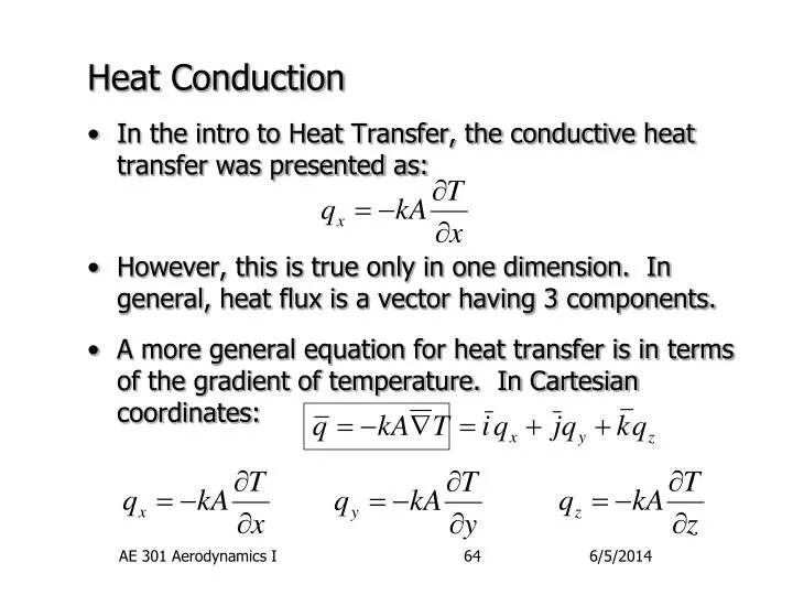
Heat Conduction • In the intro to Heat Transfer, the conductive heat transfer was presented as: • However, this is true only in one dimension. In general, heat flux is a vector having 3 components. • A more general equation for heat transfer is in terms of the gradient of temperature. In Cartesian coordinates: AE 301 Aerodynamics I
Heat Conduction (cont.) • Since we will be dealing with other coordinates also, realize that the gradient takes on other forms: Cartesian Cylindrical Spherical AE 301 Aerodynamics I
Heat Diffusion Equation • To develop a generalized governing law for heat conduction, we begin by consider the fluxes in an element as shown: AE 301 Aerodynamics I
Heat Diffusion Equation (cont.) • A statement of energy conservation for this control mass (similar to the 1st Law) would be: • Lets consider this statement term by term. First, the rate of change of energy: AE 301 Aerodynamics I
Heat Diffusion Equation (cont.) • Note that this equation uses and thus assumes constant pressure processes. • Next consider the heat generation term: • Sources of heat generation will be: electrical resistance, chemical reactions, nuclear reactions, or even radiation absorption like in a microwave. AE 301 Aerodynamics I
Heat Diffusion Equation (cont.) • Lastly, consider the heat flux through the element: AE 301 Aerodynamics I
Heat Diffusion Equation (cont.) • However, using the definition of qx, qy, and qz this can be rewritten as: • Finally, putting all these together, we get the heat diffusion equation: • Note that this is a 2nd order differential equation! AE 301 Aerodynamics I
Heat Diffusion Equation (cont.) • One common simplification of this equation is to assume that the material conductivity, k, is independent of position.This is valid if: • objects are made of a single material • k is not a strong function of T or T is nearly constant • In this case, the diffusion equation can be written as: • where AE 301 Aerodynamics I
Heat Diffusion Equation (cont.) • In the three coordinate systems of interest, the Laplace operator takes the form: Cartesian Cylindrical Spherical AE 301 Aerodynamics I
Heat Transfer Boundary Conditions • Since heat conduction problems involve differential equations, we need to consider the different types of boundary conditions. • In general, BC’s will be one of 4 types: • Fixed temperature: • T(xw,t) = Ts • Fixed heat flux • -k(dT/dx)xw=q”s Ts T(x,t) xw q”s T(x,t) AE 301 Aerodynamics I
Heat Transfer BC’s (cont) • Adiabatic Wall • -k(dT/dx)xw=0 • Convectively cooled • -k(dT/dx)xw=h(T -Ts) • Those of you who remember your Diff. Eq. Will recognize the first BC as a Dirichlet type, the next two as Neumann type, and the last as being mixed! q”s=0 T(x,t) xw Ts T(x,t) T AE 301 Aerodynamics I
1-D, Steady State Heat Transfer • In this chapter we will consider steady state heat transfer in one dimension. • As a result we can set the left hand side of our governing equation to zero: • The direction of heat flux will either be axial as in either the X or Z directions, or will be radial in the R direction. • We will also consider situations which are really multidimensional, but which can be well modeled with 1-D approximations. AE 301 Aerodynamics I
The Planar Wall • The first case of interest is the planar wall made of a single material as sketched. • We will not consider heat generation at first, so and the governing equation is just: • Another way to state this equation is: • Or T k A TS1 TS2 q x L AE 301 Aerodynamics I
kA kB kC LA LB LC The Planar Wall (cont) • A more complicated version of this problem is to combine multiple walls of different materials. • For each wall section we have: • But, it must also be true that • since energy is not stored inside the wall. T TS1 T2 T3 TS4 x AE 301 Aerodynamics I
The Planar Wall (cont) • This give three equations, and 3 unknowns (qx, T2, T3) if the two wall temperatures are given (TS1,TS2). • Solving for the qx yields: • This result can be generalized to any multilayer composite wall by introducing the concept of thermal resistance, Rt. • Thermal resistance plays the role in heat conduction as electrical resistance does in electrical conduction. AE 301 Aerodynamics I
The Planar Wall (cont) • Using an analogy to flow of electrical current, if the temperature change is the potential difference and q the flux rate, then: • The total resistance offered by this composite wall is similar to resistors in series: AE 301 Aerodynamics I
kB kA kD LB kc LA LD Lc The Planar Wall (cont) • This electrical analogy can be extended to other situations such as the wall shown. • This case resembles having resistors in series and parallel: • The resistance in this case is give by: AE 301 Aerodynamics I
The Planar Wall (cont) • And the net heat flux through the wall is just • A common way of expressing the effect of a composite wall is to use the Overall Heat Transfer Coefficient, U, defined by: • By comparison with the previous equation, it is obvious that : AE 301 Aerodynamics I
The Planar Wall (cont) • Lastly, don’t confuse the thermal resistance, Rt, with the “R” factor quoted for many common construction materials. • The “R” factor used in the construction industry is defined by: • where L is the insulation thickness in inches and k the material conductivity in BTU inches/(hr ft2oF). • Thus the “R” factor is the same as 1/U, but with British units. AE 301 Aerodynamics I
Contact Resistance • One assumption that has been made in the previous development is that heat flow easily between the different layers of material. • In fact, when two solids are in contact, their surface roughness results in voids separating the two materials. • How easily heat flows between the two materials then depends upon the amount of direct contact between them and the fluid filling the gaps. TA TB Voids AE 301 Aerodynamics I
Contact Resistance (cont) • To account for this effect, the Contact Resistance is defined by: • Unfortunately, it is very difficult to accurately predict the contact resistance and experimentation is usually necessary. • Factors which effect the how much contact resistance there is are surface preparation, contact pressure and the void fluid. • Two polished surfaces will make better contact, thus reducing resistance from the voids. AE 301 Aerodynamics I
Contact Resistance (cont) • Joining two materials by force increases the contact area through the surface by the deformation of the faces under load - thus reducing resistance. • Filling the voids with more conductive fluids such as oil or thermal greases reduces the resistance of the voids themselves. • Finally, placing a thin foil of a highly ductile and conductive material such as lead or indium between two surfaces before joining them with force acts to effectively fill the voids. • See the book for typical thermal contact resistance values. ES 312 – Energy Transfer Fundamentals
Radial Flow - Cylinders • The next case of interest is the radial flow of heat in a cylindrical system. The best instance of this case is heat loss from a pipe. • Without heat generation and with k=constant, the governing eqn. is: • Another way to state this equation is to multiply by r and combine terms: r z AE 301 Aerodynamics I
Radial Flow - Cylinders (cont) • This result is consistent with applying Fourier’s Law to the case but letting the area be a function of r: • By separating the variables and integrating: • Or: r2 r1 TS2 L TS1 AE 301 Aerodynamics I
TS1 TS2 r1 r2 Radial Flow - Cylinders (cont) • Or using the concept of thermal resistance: • Now think of the consequences of these results. • First, the temperature does not vary linearly, rather it varies with the natural logarithm of r. • Second, while the heat rate is constant, the heat flux is not, but varies as 1/r. AE 301 Aerodynamics I
r3 r2 r4 r1 TS1 TS2 Radial Flow - Cylinders (cont) • For composite radial layers, the situation is analogous to the composite planar wall. • Thus, for a pipe made of steel coated with a layer of fiberglass and then plaster: • Also, contact resistance will occur in radial systems as in planar walls. AE 301 Aerodynamics I
Radial Flow - Spheres • Radial heat flow in spheres is qualitatively similar to that in cylinders, but the flux area varies as r2. • Thus, Fourier’s Law is: • And after integrating you get: • Composite layers are handled as in the previous two cases. AE 301 Aerodynamics I
Convection Boundaries • All the cases considered thus far have assumed the surface temperatures are known. • In general, however, the temperature of the surrounding fluid is knows, and hopefully the convective heat coefficient, h. • Using the concept of thermal resistance to Newton’s Law of convective cooling shows that: h T TS AE 301 Aerodynamics I
Convection Boundaries (cont) • Thus, for cooling on a planar wall: • While for a pipe: h1 h2 T,1 k T,2 L r2 r1 h1 k T,1 h2 T,2 AE 301 Aerodynamics I
r2 h2 r1 k Critical Radius of Insulation • An unusual situation arises when applying insulation to a pipe of small radius. • If only the insulation layer and the convective process on the outer surface are considered, the thermal resistance is: • The conductive term above increases with r2, while the convective term decreases with r2. AE 301 Aerodynamics I
Rtot Rt,cond Rt,conv r1 rcr r2 Critical Radius of Insulation (cont) • Thus, a plot of Rtot versus r2 might look like: • The radius at which Rtot reaches a minimum is called the critical radius of insulation, rcr. • Below this radius, the addition of insulation is counter productive since the increase in the outer surface area (where convection occurs) is more significant than the insulating properties of the material. AE 301 Aerodynamics I
Critical Radius of Insulation (cont) • To find the rcr, we find the minimum of this curve: • Or simply: • Two notes: • First, for the insulation to be effective, the outer radius might have to be much greater than rcr. As a result, thin pipes are often left un-insulated! • Second, for some cases rcr < r1, i.e. any insulation thickness is effective. AE 301 Aerodynamics I
Heat Generation - Plane Walls • Let’s revisit the plane wall case, but this time include heat generation, . • The governing equation in this case is: • Integrating this equation twice yields a quadratic equation in x with two unknown constants of integration: • The constants must be determined by applying the appropriate boundary conditions. AE 301 Aerodynamics I
To Ts Ts T -L’ L’ x Heat Generation - Plane Walls (cont) • Let’s consider the simplest case possible, that where the temperature on both walls are equal at Ts. • Symmetry dictates that C1=0 and to have T=Ts at x=L’ (half thickness): • Note that C2 is also equal to the temperature at the center of the wall, T0. • Thus the temperature variation in the wall is given by: AE 301 Aerodynamics I
Ts2 T(x) Ts1 -L’ L’ Heat Generation - Plane Walls (cont) • In the more general case where the two surface temperatures are at different values, Ts,1 and Ts,2, the solution is: • Which looks like: AE 301 Aerodynamics I
Heat Generation - Radial Systems • Radial systems are very similar. The governing equation is: • Which after integrating twice yields: • Once again, symmetry requires C1 = 0 and C2 must equal centerline temperature and: R Ts To AE 301 Aerodynamics I
Heat Generation - Radial Systems (cont) • Substitution then yields the result that: • In the more general case shown below, the solution is: • Care to prove it? Ts,2 r2 r1 Ts,1 Ts,1 AE 301 Aerodynamics I
Heat Generation with Convection • Now let’s add surface convection into these two problems. • First, we would like to find the total heat flux out of the surface. From our previous results: Plane Wall Radial System AE 301 Aerodynamics I
Heat Generation with Convection (cont) • In retrospect, this result makes sense - the heat flux out must equal the heat generated within! • However, this heat to the wall must be carried away by convection (or radiation, possibly). • Thus: • Notice how these results are independent of the internal temperature profile! Plane Wall Radial System AE 301 Aerodynamics I
T h Ts A Extended Surfaces • From considering the critical radius of insulation, we saw the importance of surface area when determine the total heat transfer in a combined conduction/ convection system. • In many surfaces the rate of heat transfer can be enhanced by increasing surface area through the use of extended surfaces or “fins” • Consider the case shown below: T h Ts A AE 301 Aerodynamics I
Extended Surfaces (cont) • The addition of fins can greatly increase the total convective surface area. • However, realize that this added surface area is not as effective as the original since T decreases from the base temp, Tb, along the length of the fin! • Since the heat loss from the fin is proportional to the difference (T(x) - T), the base of the fin is more effective than the root. • To calculate the net heat flux, we need to find T as a function of x. Tb T(x) T x AE 301 Aerodynamics I
Extended Surfaces (cont) • This problem is at least 2 dimensional. However a very good approximation involves considering heat flux in only one dimension - base to tip. • Heat flux normal to this direction can be modeled as heat loss (negative ) which is due to convection. • To see this, consider the following fin geometry: • Let Ac be the fin tip area and P the length of the perimeter of this area. • Then dx Ac P AE 301 Aerodynamics I
Extended Surfaces (cont) • The governing equation for this quasi 1-dimensional problem is then: • This problem can be notationally simplified by letting: • To get: which has the general solution: AE 301 Aerodynamics I
Extended Surfaces (cont) • To solve for the two constants A and B, we need two boundary conditions. • At the base, Tx=0 = T0, or • At the other end, the tip, the best B.C. would include the effect of tip heat convection, or: • In practice, it is more reasonable that no heat is lost through the tip both because Ac is small and the temperature there is close to T. I.e. AE 301 Aerodynamics I
Extended Surfaces (cont) • With this “insulated end” B.C., the solution for A and B yields: • Of course, the temperature distribution is secondary. What we really want is the fin heat loss rate: AE 301 Aerodynamics I
Fin Effectiveness and Efficiency • When designing fins, or deciding what fin to use, it is useful to have some parameters for comparison. • For fins, there are two parameters commonly used: effectiveness and efficiency. • Fin effectiveness, : the ratio of the fin heat transfer rate to the heat transfer rate that would exist without the fin. • Fin effiiciency, : the ratio of the fin heat transfer rate to the ideal case where T(x) = T0 all along the fin length. • Fin effectiveness will tell us how much more effective having the fin is over not having it. • Fin efficiency will tell us whether it makes the optimum use of material. AE 301 Aerodynamics I
Fin Effectiveness and Efficiency (cont) • For the case just considered, the effectiveness would be: • Note that for long fins (tanh(mL)1), then three things improve fin effectiveness: • A high material conductivity. Pretty obvious! • A low fluid convectivity. This does not mean that you want h low, just that fins are more commonly used when h is small as in natural convection and/or gasses versus liquids. • A large ratio of tip area to tip perimeter, Ac/P. Thus a wide, thin fin is preferable. Another way to say this is that you would rather have two thin fins then one twice as thick AE 301 Aerodynamics I
Fin Effectiveness and Efficiency (cont) • The fin efficiency for this case is: • This result indicates two things. • The highest efficiency, 1, is achieved for a short fin since tanh(mL)mL as L is decreased. • The fin efficiency decreases to a value of zero as the length increases. • This is because the region near the tip, where TT, does not contribute as much as the base sections. AE 301 Aerodynamics I
Other Fin Shapes • The book gives the results for span efficiency for other type fins on pages 45 and 46. • Note that the first case shown is the one we just solved, but using a corrected length, Lc, not L. • This slight change improves the comparison to experiment since the tip is not really insulated! • Also note that all these solutions just provide the find efficiency and the fin wetted area, Af. • To get fin effectiveness, use: AE 301 Aerodynamics I
Fin Thermal Resistance • When dealing with complex thermal flow situations, it is useful to fall back to the electrical analogy. • For fins, the thermal efficiency is defined by: • However, also note that the fin effectiveness is related to the fin thermal efficiency by: • Thus use the chart to get efficiency, then from that find the fin effectiveness and the Rf. AE 301 Aerodynamics I