Download
1 / 87
1.66k likes | 3.13k Vues
Heat-conduction/Diffusion Equation. Outline. This topic discusses numerical solutions to the heat-conduction/ diffusion equation: Discuss the physical problem and properties Examine the equation Approximate solutions using a finite-difference equation Consider numerical stability Examples.

E N D
Outline This topic discusses numerical solutions to the heat-conduction/ diffusion equation: • Discuss the physical problem and properties • Examine the equation • Approximate solutions using a finite-difference equation • Consider numerical stability • Examples
Outcomes Based Learning Objectives By the end of this laboratory, you will: • Understand the heat-conduction/diffusion equation • Understand how to approximate partial differential equations using finite-difference equations • Set up solutions in one spatial dimension • Understand the implementation of insulated boundaries
Motivating Example Suppose you have a metal bar in contact with a body at 100 °C • If the bar is insulated, over time, the entire length of the bar will be at 100 °C 0 °C 100 °C
Motivating Example At time t = 0, one end of the bar is brought in contact with a heat sink at 0 °C 0 °C 100 °C
Motivating Example At the end closest to the heat sink, the bar will cool rapidly; however, the cooling is not uniform 0 °C 100 °C
Motivating Example Over time, however, the temperature will drop linearly from 100 °C to 0 °C across the bar 0 °C 100 °C
The Heat-conduction/Diffusion Equation The equation that describes the change in temperature over time is given by the partial differential equation where u(x, t) is a real-valued function of space and time and k > 0 is the thermal diffusivity coefficient heat conduction diffusivity coefficient diffusion
The Laplacian Equation The heat-conduction/diffusion equation is a time-independent version of Laplace’s equation where u(x) is a real-valued function of space
The Laplacian Operator The Laplacian operator depends on the dimensions of space argument • In one dimension, and therefore • In two dimensions, and therefore • In three dimensions, and therefore
The Laplacian Equation In Laboratory 1, we saw that the only solution to Laplace’s equation in one dimension with boundary values is a straight line The solution of is
The Laplacian Operator Notice if that u(x, t) already satisfies Laplace’s equation, then or That is, if a solution already satisfies Laplace’s equation, it will not vary over time • In one dimension, if the bar is already linearly varying from 0 to 100, placing a heat source and sink at each end will not change the temperature
Applications Applications of the heat-conduction/diffusion equation include: • Heat equation • Fick’s laws of diffusion • Thermal diffusivity in polymers Oleg Alexandrov Steven Byrnes
Rate of Change Proportional to Concavity In one dimension, what does this equation mean? • Recall we assumed that k > 0 • If the function u is concave up at (x, t), the rate of change of u over time will be positive • That is, it will become less concave up • If the function u is concave down at (x, t), the rate of change of u over time will be negative • That is, it will become less concave up
Rate of Change Proportional to Concavity We can see this visually: • If the function u is concave up at (x, t), the rate of change of u over time will be positive
Rate of Change Proportional to Concavity We can see this visually: • If the function u is concave down at (x, t), the rate of change of u over time will be negative
Rate of Change Proportional to Concavity We can see this visually: • Of course, a function may be concave up and down in different regions Ultimately, the concavity tends to disappear—that is, as time goes to infinity, u(x, t) becomes a straight line…
Examples Consider heat conduction problem: • A bar initially at 5 °C with one end touching a heat sink also at 5 °C • At time t = 0, the other end is placed in contact with a heat source at80 °C
Examples As time passes, the bar warms up
Examples A plot of the temperature over time across the bar is given by this solution: • The end placed in contact with the 80 °C heats up faster than points closer to the heat sink • As the concavity becomes smaller, the rate of change also gets smaller
Examples A plot of the temperature over time across the bar is given by this solution: • The end placed in contact with the 80 °C heats up faster than points closer to the heat sink • As the concavity becomes smaller, the rate of change also gets smaller
Examples Consider another example: • A bar initially at 100 °C is placed at time t = 0 in contact with a heat source of 80 °C at one end and a heat sink at 5 °C
Examples The ultimate temperature will be no different: • A uniform change from 80 °C down to 5 °C
Example A plot of the temperature over time across the bar is given by this solution: • Both ends drop from 100 °C however, the centre cools slower than does the bar at either end point
Example A plot of the temperature over time across the bar is given by this solution: • Both ends drop from 100 °C however, the centre cools slower than does the bar at either end point
Rate of Change Proportional to Concavity Ultimately, the concavity tends to disappear—that is, as time goes to infinity, u(x, t) becomes a straight line… Important note: • This statement is onlytrue in one spacial dimension • In higher spacial dimensions, u(x, t) will approach a solution to Laplace’s equation in the given region
Approximating the Derivative Questions: • How do we approximate partial derivatives? • What are the required conditions?
Approximating Partial Derivatives Recall our approximations of the derivatives: In this case, however, we are dealing with partial derivatives
Approximating Partial Derivatives If you recall the definition of the partial derivative, we focus on one variable and leave the other variables constant To ensure clarity: • h is used to indicate small steps in space • Dt is used to indicate a small step in time
Approximating Partial Derivatives The obvious extension is to define
Approximating Partial Derivatives If we substitute the second into the heat-conduction/diffusion equation, we or
Similarity with IVPs If this looks familiar to you, it should: Recall Euler’s method: if y(1)(t) = f (t, y(t)) and y(t1) = y1, it follows that The slope at (t1, y1)
Approximating the Second Partial Derivative The next step is to approximate the concavity We will use our 2nd-order formula: to get
Approximating the Second Partial Derivative There is only one small interesting issue: • What happens if the coefficient is very large? • It should be obvious; however, we will be approximating these at discrete points:
Approximating the Second Partial Derivative There is only one small interesting issue: • Consider the total sum: • If , the contribution from the boundary conditions will always increase; thus, for stability, we require
Initial and Boundary Conditions For a 1st-order ODE, we require a single initial condition
Initial and Boundary Conditions For a 2nd-order ODE, we require either two initial conditions or a boundary condition: Time variables are usually associated with initial conditions Space variables are usually associated with boundary conditions
Initial and Boundary Conditions For the heat-conduction/diffusion equation, we have: • A first-order partial derivative with respect to time • A second-order partial derivative with respect to space
Initial and Boundary Conditions For the heat-conduction/diffusion equation, we require: • For each space coordinate, we require an initial condition for the time • For each time coordinate, we require a boundary conditions for the space
Initial and Boundary Conditions In this case, we will require an initial value for each space coordinate • Keeping in the spirit of one dimension: • If we were monitoring the progress of the temperature of a bar, we would know the initial temperature at each point of the bar at time t = t1 • If we were monitoring the diffusion of a gas , we would have to know the initial concentration of the gas
Initial and Boundary Conditions Is a one-dimensional system restricted to bars and thin tubes? • Insulated wires, impermeable tubes, etc. No, many systems where two spacial dimensions are significant larger than one may be approximated by a one-dimensional system away the boundaries • Consider the effect of a thin insulator between twomaterials that have approximately uniformtemperature • Consider the diffusion of particles across amembrane separating liquids with differentconcentrations In all such cases, it may be able toapproximate the system as a one-dimensionalsystem
Approximating the Solution Just as we did with BVPs, we will divide the spacial interval [a, b] into nx points or nx – 1sub-intervals
Approximating the Solution Just as we did with BVPs, we will divide the spacial interval [a, b] into nx points or nx – 1sub-intervals • The initial state at time t = t1 would be defined by a function uinit(x) where uinit:[a, b] → R
Approximating the Solution As with Euler’s method, we will attempt to approximate the solution u(x, t) at discrete times in the future • Given the state at time t = t1, approximate the solution at time t = t2
Approximating the Solution Never-the-less, we must still determine the 2nd-order component • This requires two boundary values at a and b
Approximating the Solution Indeed, at each subsequent point, we will require the boundary values • Over time, the boundary values could change
Approximating the Solution Therefore, we will need two functions abndry(t) and bbndry (t) • At each step, we would evaluate and determine two the boundary conditions
Approximating the Solution Therefore, we will need two functions abndry(t) and bbndry (t) • We would continue from our initial time tinitial and continue to a final time tfinal
Approximating the Solution Like the spatial dimension, we would break the time interval into nt discrete points where
Approximating the Solution Therefore, we will need two functions abndry(t) and bbndry (t) • We would continue from our initial time tinitial and continue to a final time tfinal