Download
1 / 85
850 likes | 1.03k Vues
The Fine-Tuning of the Universe for Scientific Technology and Discoverability. PART I: BACKGROUND. Review of Anthropic Fine-tuning evidence.

E N D
The Fine-Tuning of the Universe for Scientific Technology and Discoverability
Review of Anthropic Fine-tuning evidence The anthropic fine-tuning refers to the fact that the basic structure of the universe must be precisely set for life to exist, particularly embodied conscious agents (ECAs). The fine-tuning comes in three types: Fine-tuning of mathematical form of the laws of physics Fine-tuning of the fundamental parameters of physics Fine-tuning of the initial conditions of the universe Most of the discussion in the literature has been on (2), the fine-tuning of the fundamental parameters of physics.
Fine-tuning of Fundamental Parameters Question: “What are the fundamental parameters of physics?” Answer: They are the fundamental numbers that occur in the laws of physics. Many of these must be precisely adjusted to an extraordinary degree for ECAs to exist.
The Gravitational constant – designated by G -- determines the strength of gravity via Newton’s Law of Gravity: F = Gm1m2/r2, where F is the force between two masses, m1 and m2, that are a distance r apart. Increase or decrease G and the force of gravity will correspondingly increase or decrease. (The actual value of G is 6.67 x 10⁻¹¹ Nm2/kg2.) Example: Gravitational Constant m1 r m2
Dimensionless Expression of Strength of Gravity The gravitational constant G has units (e.g., in the standard international system it is G is 6.67 x 10⁻¹¹ Nm2/kg2 ). Physicists like to use a measure of the strength of gravity that does not have units. A standard choice is: αG = G(mp)2/ℏc, where mpis the mass of the proton, ℏ is the reduced Planck’s constant, and c is the speed of light. Other parameters are also usually expressed in dimensionless form.
Example of Fine-Tuning: Dark Energy Density The effective dark energy density helps determine the expansion rate of space. It can be positive or negative. Unless it is within an extremely narrow range around zero, the universe will either collapse or it will expand too rapidly for galaxies and stars to form. How fine-tuned is it?
Answer: In the physics and cosmology literature, it is typically claimed that in order for life to exist, the cosmological constant must fall within at least one part of 10120– that is, 1 followed by 120 zeros -- of its theoretically natural range. This is an unimaginably precise degree of fine-tuning.
Dark Energy Density: Radio Dial Analogy WKLF: You must tune your dial to much less than a trillionth of a trillionth of an inch around zero. +15 billion light years. -15 billion light years.
Summary of Evidence Biosphere Analogy: Dials must be perfectly set for life to occur. (Dials represent values of fundamental parameters. Illustration by Becky Warner, 1994.)
Review of Multiverse Explanation The so-called “multiverse hypothesis” is the most common non-theistic explanation of the anthropic fine-tuning. According to this hypothesis, there are an enormous number of universes with different initial conditions, values for the fundamental parameters of physics, and even the laws of nature.Thus, merely by chance, some universe will have the “winning combination” for life; supposedly this explains why a life-permitting universe exists.
Observer Selection Effect The Observer Selection Effect is crucial to the multiverse explanation. According to this idea, observers can only exist in universes in which the laws, constants, and initial conditions are life-permitting. Therefore, it is argued, it is also no coincidence that we find ourselves in an observer-permitting universe.
Multiverse Hypothesis Humans are winners of a cosmic lottery:
Many Planets Analogy Given that the universe contains a huge number of planets, it is no surprise that there is a planet which orbits just the right star and is just the right distance from the star for life to occur. Further, it is no surprise that we find ourselves on such a planet, since that is the only kind of planet creatures like us could exist on.
Testing the Theistic Explanation against the Multiverse Explanation Features of the universe that confirm divine purpose over a naturalistic multiverse will consist of features of the universe that meet the following conditions: (1) We can glimpse how they could help give rise to a net positive moral value – and hence it would not be surprising that an all-good God would create a universe with these features; (2) They cannot be explained by an observer-selection effect . (3) They are very coincidental (surprising, epistemically improbable) under the non-theistic multiverse.
Discoverability Our ability to discover the nature of the universe, which prominent scientists such as Albert Einstein and Eugene Wigner considered to border on the “miraculous,” seems to meet the three criteria: Criterion (1): We normally take discovering the nature of our universe to be of value – either as intrinsically valuable or because it helps us develop technology. Therefore, it would not be surprising under theism that the universe would be structured so that it exhibits a high degree of discoverability.
Criteria (2) – (3) Criteria (2) – (3): There seems to be no necessary connection between a universe being life-permitting and its being discoverable beyond that required for getting around in the everyday world. Thus if the proportion of life-permitting universes that are as discoverable as ours is really small, it would be very improbable under a multiverse hypothesis that as generic observers we would find ourselves in such a universe. I will provide quantitative evidence that this proportion is small.. Life-permitting universes that not highly discoverable. A life-permitting universe that is highly discoverable
PART II: CASES OF DISCOVERABILTY In the following slides, I will focus on the cases of discoverability involving the fundamental parameters of physics since we can potentially get a quantitative handle on the degree of discoverability in these cases. However, a significant case for discoverability can be made from the fact that the laws of nature have the right form so that we can discover them. This has been pointed out by Eugene Wigner in his famous piece “The Unreasonable Effectiveness of Mathematics in the Natural Sciences” (1960), and recently elaborated in some detail by Mark Steiner in his Mathematics as a Philosophical Problem(1998).
Examples of Fine-tuning of Laws • Hierarchical simplicity • Quantization Technique • Gauge (local phase) invariance technique 4. Structure of quantum mechanics itself (complex numbers, measurement rule, etc.) Eugene Wigner: “The miracle of the appropriateness of the language of mathematics for the formulation of the laws of physics is a wonderful gift which we neither understand nor deserve” (1960). Einstein: “The most incomprehensible thing about the universe is that it is comprehensible."
Two Types of Fine-tuning for Discoverability To get a quantitative handle on how coincidental the discoverability of the universe is, for each fundamental parameter of physics, I consider the effects on discoverability of varying it. By doing this, I have found that there are two types of fine-tuning for discoverability:
Type 1: Livability/Discoverability-Optimality Fine-tuning Livability/Discoverability-Optimality Fine-tuning. This sort of fine-tuning of a parameter occurs if given the basic overarching principles of physics and the current mathematical form of the laws: (i) the parameter is within its livability-optimality range (the range between the thin solid vertical lines); (ii) The parameter falls into that part of the livability-optimality range that maximizes discoverability (range between thin dashed lines). This is shown in the figure below, with the star representing the actual value of the parameter in question: Note: The region between the two thick black lines is the life-permitting range. As far as I can tell, all fundamental parameters seem to be fine-tuned in such a way as to satisfy Livability/Discoverability Optimality.
Example 1: CMB The most dramatic case that I have discovered of this kind of fine-tuning is that of the Cosmic Microwave Background Radiation (CMB). The CMB is microwave radiation that permeates space. It was caused by the big bang.
Basic Idea Behind Big Bang The visible universe began in an explosion in which all its matter and energy was condensed into a volume less than the size of a golf ball. It consisted mostly of very intense light in the form of photons and particle/anti-particle pairs. Since that time, the universe has been expanding, causing it to cool.
Why Microwave Radiation? Blue wavelength • As the universe expands, a photon’s wavelet is stretched because of the expansion of space between the beginning and end of the wavelet. This causes the distance between the crests to get longer and longer. • Thus if a photon of light starts off with a wavelength (~450nm) corresponding to blue light, it’s wavelength will get longer and longer. If the universe expands enough, the wavelength will be stretched into the microwave region of the spectrum (~1mm – 10mm). Microwave Wavelength
Significance of the CMB The CMB tells us critical information about the large scale structure of the universe: “The background radiation has turned out to be the ‘Rosetta stone’ on which is inscribed the record of the Universe’s past history in space and time.” (John Barrow and Frank Tipler, The Cosmological Anthropic Principle, 1986, p. 380).
Optimizing CMB • Much of the information in CMB is in very slight variations in its intensities of less than one part in 100,000 in different parts of the sky. • Since it is already fairly weak, this implies that within limits, the more intense it is, the better a tool it is for discovering the universe.
CMB and Baryon/Photon Ratio Intensity of CMB depends on baryon to photon ratio: ηbγ = (#baryons/#photons) = (#protons + #neutrons per unit volume)/(#photons per unit volume). Prediction of Livability/Discoverability-optimality Fine-tuning: Within the range that ηbγ does not influence livability or other types of discovery, its value is such as to maximize the intensity of the CMB since this would maximize discoverability.
Prediction Correct! Note that the intensity of the CMB is maximal when ηbγ/ηbγ0 = 1: that is, when the baryon to photon ratio is the same as in our universe. Plot of the intensity of the cosmic microwave background radiation (CMB) versus the baryon to photon ratio. CMB/CMB0 represents the intensity of the CMB in the alternative universe compared to our universe, and ηbγ/ηbγ0 represents the baryon to photon ratio in the alternative universe compared to that in our universe.
*Example 2: Weak Force (α w) • The primary role the weak force plays in the universe is the interconversion of protons to neutrons. Potassium 40 (K40) and Carbon 14 (C14) both form the basis of two important dating techniques. Both decay via the weak force. Their decay rate ∝ α w2. • Thus, increase the weak force by ten-fold, the decay of rate of potassium-40 would be one hundred times as large, making the amount of K40 in the earth far below the range of detectability; this would render K40 dating useless for dating. Further, the life-time of C14 would be 57 years, instead of 5,700 years. This would make C14 dating useless for artifacts much older than 300 – 400 years old. • Note: Particularly in the case of C14, decreasing the weak force does not allow any new dating technique that could replace C14 to become available.
Weak Force -- Continued The neutrino interacts with other particles via the weak force. Because of this interaction is so weak, neutrinos are very difficult to detect. However, neutrinos carry important information about nuclear processes in the interior of the earth and stars, information that no other known form of radiation carry. Decrease weak force by 10-fold, it would be virtually impossible to detect neutrinos from the earth, sun, and supernovae. Already, detectors are very expensive and the number of neutrinos detected is barely above background noise. require an enormous amount of fluid. Thus, when both radioactive dating and neutrino detection are taken into account, the weak force seems to fall into the discernible-discovery-optimal range.
Type 2: Tool Usability Fine-tuning The second type of “fine-tuning” is that for having enough usable tools to make the universe as discoverable as our universe is. To explicate this fine-tuning requires defining some terms.
Tools and Discoverability Constraints • A Tool of Discoveryis either some artifact or feature of the universe that is used to discover the domain. For example, a light microscope is a tool used to discover the structure of living cells. • A Tool Usability Constraintis a non-anthropic/livability constraint that must be met in order for the tool to be usable. These constraints constitute necessary, though not sufficient, conditions for usability. For example, a necessary condition for the use of potassium-argon dating is that there be detectable levels of radioactive potassium 40 in the earth.
Tool Usability Constraint Range and Bounds A tool usability constraint bound on a parameter is the range of values that the parameter can have for which the tool is usable.
Two Illustrations of Concepts 1. Wood fires and the fine-structure constant. 2. Light microscopes and the fine-structure constant.
Fine-Structure Constant (α) The fine-structure constant, α, is a physical constant that governs the strength of the electromagnetic force. If it were larger, the electromagnetic force would be stronger; if smaller, it would be weaker.
Example #1: Fires and α A small increase in α would have resulted in all wood fires going out . . .
Civilization and Wood Fires . . . but harnessing fire was essential to the development of civilization, technology, and science – e.g., the forging of metals.
Explanation Why would an increase in α have this result? Answer: In atomic units, everyday chemistry and the size of everyday atoms arenot affected by a moderate increase or any decrease in α. Hence, the combustion rate of wood remains the same. In these units, however, the rate of radiant output of a fire is proportional to α2. Therefore, a small increase in α – around 10% to 40% -- causes the radiant energy loss of a wood fire to become so great that the energy released by combustion cannot keep up, and hence the temperature of the fire must decrease to below the combustion point. .
Conclusion for α and Wood Fires Upper Bound on α: The ability of embodied conscious agents (ECAs) to build open wood fires, and hence forge metals,drastically decreases if α is greater than 10% to 40% of its current value. This is represented in the figure below: the actual value of α is represented by the star. The star must fall below the dashed vertical line in order to have open wood fires. Tool = open wood fires for forging metals. Tool usability constraint –ability to ignite and maintain open wood fires. Tool usability constraint range for α – range of α for which it is possible to have open wood fires (all the values for α below the thick vertical dashed line). 0
Example 2: Microscopes and α A relatively small decrease in α would decrease the maximum resolving power of microscopes so they could no longer see cells – thus severely inhibiting, if not rendering impossible, advanced medical technology (such as the development of germ theory). As is, α is just large enough to allow us to see of 0.2 microns, the size of the smallest living cell.
*Why this Effect? • In atomic units, the speed of light = c = 1/α. Decreasing α, therefore, increases the speed of light without affecting everyday chemistry or the size of atoms. Thus, the world would look mostly the same. • The energy of a photon = E = hf, where h is Planck’s constant and f is the frequency of light. (h = 1 in atomic units). • A photon of visible light cannot have more energy than the bonding energy of typical biochemical molecules, otherwise it would destroy the molecules in an organism’s eye. This requires that for light microscopes, f < 800 trillion cycles per second. • Wavelength of light = λ = c/f. In our world, the above restriction on frequency means that λ > 0.35 microns. Since c = 1/α, as α decreases, c increases, which causes the minimum wavelength of light for a light that can be used without destroying an organism’s eye; this in turn means that the resolving power of light microscopes will decrease since their maximum resolving power is half a wavelength (λ/2).
A “Second-Order” Coincidence The only alternative to light microscopes for seeing the microscopic world is electron microscopes, which can see objects up to a thousand times smaller than can be seen by light microscopes. Besides being very expensive and requiring careful preparation of the specimen, electron microscopes cannot be used to see living things. Thus, it is quite amazing that the resolving power of light microscopes goes down to that of the smallest cells (0.2 microns), but no further. If it had less resolving power, these cells could not be observed alive.
Summary 0 0 Top Figure: The star represents the current value of α and thin dashed line represents the lower bound of α for which the light microscope would be usable for seeing all living cells. Bottom Figure: Combines the wood-fire upper bound and the light microscope lower bound for α. The coincidence is that the wood-fire upper bound falls above the actual value of α and the light-microscope lower bound falls below.
Main Argument Define {Ti0} as the set of tools that we use in our universe to discover various physical domains. Given this definition, the main argument can be summarized as follows: • It is highly epistemically improbable (i.e., very surprising) under naturalism that every member of {Ti0} is usable • It is not surprising under theism that every member of {Ti0} is usable. • Therefore, by the likelihood principle of confirmation theory, the usability of {Ti0} strongly confirms theism over naturalism.
Example 3: Electric Transformers and α • In atomic units, the strength of a magnetic field produced by a current or magnetic dipole in a ferromagnetic substance is proportional to α2. • One Consequence: Decreasing α would require that transformers be proportionally larger; this would cause a proportionate increase in loss of energy by hysteresis – already a limiting factor.
Example 4: Length of Year and α 1. Length of year determines length of seasons. 2. Importance of seasons: (a) instills planning for future; (b) allows for dating by means of stratigraphy (tree rings, lake beds, coral reefs, ice cores, etc.); (c) helps in keeping historical records. To be effective in the above ways, the seasons must not be too short or too long.
Length of Year and α -- continued L(year) ∝ α-11/2 (Lightman, 1984, Eq. 22, p. 213). Increase α by a factor of 3, a year becomes less than an earth day. Decrease α by a factor of 5, a year becomes greater than 10,000 earth years. Both cases would eliminate usefulness of seasons mentioned above, without giving rise to anything to replace their role in discoverability.
*Example 5: Parallax and α By measuring the angle p’’, one can determine the distance to a star using the formula: 1au = distance from sun to earth = dsin(p’’). Therefore, d = 1au/sin(p’’).