Download
1 / 12
120 likes | 252 Vues
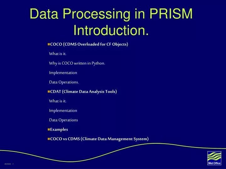
Data Processing in PRISM Introduction. COCO (CDMS Overloaded for CF Objects) What is it. Why is COCO written in Python. Implementation Data Operations. CDAT (Climate Data Analysis Tools) What is it. Implementation Data Operations Examples

E N D
Data Processing in PRISM Introduction. COCO (CDMS Overloaded for CF Objects) What is it. Why is COCO written in Python. Implementation Data Operations. CDAT (Climate Data Analysis Tools) What is it. Implementation Data Operations Examples COCO vs CDMS (Climate Data Management System)
What is COCO? • Processing library written in Python which reads and manipulates netCDF data conforming to the Climate and Forecast (CF) metadata conventions. • Provides an implementation for the ADT specification describing the encapsulated CF metadata read in from disk. • Defines the properties and set of operations for manipulating encapsulated CF metadata objects in memory. • Conversion of the CF metadata objects between files of different formats possible.
Why Python? • Influence of CDAT/CDMS which is written in Python. • Dynamically typed - ease of use for scientists. • Enables you to base structure of code on object type rather than on actions - convenient way to store CF metadata with data. • Compatability with other languages - easy to combine with other software libraries using tools to automate the task e.g SWIG. • Efficiency and high performance may be achieved via C code - Python’s Numeric library is such an example.
COCO Implementation • A space construct defines a grid of zero or more dimensions. The dimensions are the only information which is always present in the space construct >>> grid = SpaceConstruct((96,73)) • Identification of variables using standard names. >>> grid.standard_name = ‘temperature_on_theta_levels’ • Units attribute required for all variables that represent dimensional quantities. >>> grid.units = ‘K’ • Space construct may also contain coordinate constructs, data and attributes • A coordinate construct has a list of dimensions and axis names, coordinate data, bounds and properties.
COCO Implementation (cont.) • A coordinate construct has a name when in a space construct. The axis names are chosen when the space construct is created. >>> grid.getAxis() # [‘axis1’, ‘axis2’] >>> coord = grid.getCoord(‘axis2’) • The axes X,Y,Z,T have special status in CF and are identified by units attribute of the coordinate construct. >>> coord.units = ‘degrees_east’ >>> grid.putCoord(coord) >>> grid.getCoord(‘X’) • Description of intervals and cells done via the get/putBounds feature of the coordinate construct.
COCO Implementation (cont.) • Description of climatological statistics >>> grid.setCellMethod(‘X’, ‘mean’) • Data in space constructs has dimensions corresponding to axes in the order specified, with each axis being arranged in the sense with increasing coordinate values. >>> grid.putValue(MaskedArray(zeros([96,73])), axis=‘yx’) • Any construct which contains coordinate data but is not a coordinate variable is known as an auxiliary coordinate construct. Auxilliary coordinates can be multidimensional.
COCO Data Operations • There are the following major operations for producing new space constructs with modified attributes/coordinates. • Subspace extraction - selects a portion of each axis. • Collapse - mean, max, min along dimension etc.. • Interpolation - changes gridpoint coordinates along axis. • Lumping - changes gridcell boundaries along axis. • Merging - e.g replace lat-lon-time field with a set of timeseries. • Concatenation - combines common dimensions. • Splitting - decomposes a space construct.
What is CDAT/CDMS? • PCMDI’s Climate Data Analysis Tools focus is to access and analyse multi-dimensional distributed climate datasets. • Links together separate software subsystems and packages to form an integrated environment for solving model diagnosis problems. • Comes with a variety of user applications including command-line interaction, stand-alone scripts (applications) and a GUI. • The CDAT subsystems, implemented as modules, provide access to and management of gridded data (CDMS), array numerical operations (Numerical Python) and visualisation (VCS). • PCMDI has integrated LAS (Live Access Server) and DODS (Distributed Oceanographic Data System).
CDMS Data Operations • When a function is performed on a variable that modifies its axes a transient variable is returned with new dimensions and axes. • variable.subRegion - extract a hyperrectangle - specified by ranges of coordinate values. • variable.subSlice - restrict variable to particular indices along one or more axes. • Various operations exist for particular interpolation. • variable.regrid for lat-lon grids. • variable.crossSectionRegrid for lat-level grids • variable.pressureRegrid for lat-pressure grids.
COCO vs. CDMS • The space construct in COCO currently uses the CDMS Variable for netCDF IO and the CDMS Axis to assist in the creation of bounds. • It is not yet decided how the library is going to be written - may decide to implement the space construct as a descendant of the CDMS Variable. • CDMS is currently being made CF compliant.
>>> file = File(‘model.nc’) >>> spaceConstructs = file.read() >>>for grid in spaceConstructs: >>> print grid.standard_name >>> x = grid.getCoord(‘longitude’) >>> y = grid.getCoord(‘Y’) >>> if grid.hasTAxis(): >>> print grid.getAlias(‘t’) >>> print grid.getAxis() >>> print grid.getCoord(‘z’).getValue() >>>simpleMeans = Collapse(spaceConstructs, method=‘mean’, axis=‘x’) >>> for grid in simpleMeans: >>> print grid.getValue().shape >>> print grid.getValue(t=‘0’,z=‘0:2’, y=‘0:2’) >>>output = File(‘model_zonal_means.nc’) >>>output.write(simpleMeans) tap time (‘time’, ‘level0’, ‘latitude’, longitude’) [30.,50.,100.,150.,200.,300.,500.,700.,850.] (22, 9, 73, 1) [[[ 216.44436646,] [ 216.53549194,]] [[ 218.09178162,] [ 218.151153503, ]]] COCO Example
VCS Example • >>>import cdms, vcs • >>>f=cdms.open(‘file.nc’) • >>>variable = f(‘tap’) • >>>w = vcs.init() • >>>w.plot(variable)