Download
1 / 23
370 likes | 928 Vues
Multimedia Compression Algorithms. Wen-Shyang Hwang KUAS EE. Outline. Introduce to Compression Lossless Compression Algorithm Lossy Compression Algorithm Image Compression Standards. Compression.

E N D
Multimedia Compression Algorithms Wen-Shyang Hwang KUAS EE.
Outline • Introduce to Compression • Lossless Compression Algorithm • Lossy Compression Algorithm • Image Compression Standards
Compression • Compression: the process of coding that will effectively reduce the total number of bits needed to represent certain information. • If compression and decompression processes induce no information loss, then the compression scheme is lossless; otherwise, it is lossy. • Basics of Information Theory • Entropyof an information source with alphabet S ={s1,s2,..,sn} is pi : probability that symbol si will occur in S. indicates amount of information contained in si, which corresponds to the number of bits needed to encode si. • The entropyspecifies the lower bound for the average number of bits to code each symbol in S
Lossless Compression • Variable-Length Coding (VLC): the more frequently-appearing symbols are coded with fewer bits per symbol, and vice versa. • Shannon-Fano Algorithm • Sort symbols according to the frequency of occurrences. • Recursively divide symbols into two parts, each with approximately same counts, until all parts contain only one symbol. • Example: Frequency count of the symbols in "HELLO"
Huffman Coding • Initialization: Put all symbols on a list sorted according to frequency. • Repeat until the list has only one symbol left: • From the list pick two symbols with the lowest frequency counts. Form a Human subtree that has these two symbols as child nodes and create a parent node. • Assign the sum of the children's frequency counts to the parent and insert it into the list such that the order is maintained. • Delete the children from the list. • Assign a codeword for each leaf based on the path from the root. The contents in the list:
Adaptive Huffman Coding • statistics are gathered and updated dynamically as data stream arrives. • increments the frequency counts for the symbols • Example:Initial code assignment for AADCCDD
Dictionary-based Coding • Lempel-Ziv-Welch (LZW) algorithm employs an adaptive, dictionary-based compression technique. • LZW uses fixed-length codewords to represent variable-length strings of symbols/characters that commonly occur together. • Example: LZW compression for string “ABABBABCABABBA" Output codes are: 1 2 4 5 2 3 4 6 1. Instead of sending 14 characters, only 9 codes need to be sent (compression ratio = 14/9 = 1.56).
Lossless Image Compression • Approaches of Differential Coding of Images: • Given an original image I(x, y), using a simple difference operator we can define a difference image d(x, y) as follows: • Due to spatial redundancy existed in normal images I, the difference image d will have a narrower histogram and hence a smaller entropy Distributions for Original versus Derivative Images. (a,b): Original gray-level image and its partial derivative image; (c,d): Histograms for original and derivative images.
Lossless JPEG • The Predictive method: • Forming a differential prediction: A predictor combines the values of up to three neighboring pixels as the predicted value for the current pixel, indicated by `X' in Figure. The predictor can use any one of the seven schemes listed in the below Table. • Encoding: The encoder compares the prediction with the actual pixel value at the position `X' and encodes the difference using one of the lossless compression techniques, e.g., the Human coding scheme.
Lossy Compression Algorithms • lossy compression • Compressed data is not the same as the original data, but a close approximation of it. • Yields a much higher compression ratio than that of lossless compression. • Distortion Measures • mean square error(MSE) 2, where xn, yn, and N are the input data sequence, reconstructed data sequence, and length of the data sequence respectively. • signal to noise ratio (SNR), in decibel units (dB), where is the average square value of the original data sequence and is the MSE. • peak signal to noise ratio (PSNR), Which measures the size of the error relative to the peak value of the signal Xpeak
Rate-Distortion Theory • Rate: average number of bits requiredto represent each source symbol. • Provides a framework for the study of tradeoffs between Rate and Distortion. Typical Rate Distortion Function. D is a tolerable amount of distortion, R(D) specifies the lowest rate at which the source data can be encoded while keeping the distortion bounded above by D. D=0, have a lossless compression of source R(D)=0 (Dmax), max. amount of distortion
Quantization • Three different forms of quantization. • Uniform: partitions the domain of input values into equally spaced intervals. Two types - • Midrise: even number of output levels (a) • Midtread: odd number of output levels (b); zero: one of output • Nonuniform: companded (Compressor/Expander) quantizer. • Vector Quantization.
Companded and Vector quantization • A compander consists of a compressor function G, a uniform quantizer, and an expander function G−1. • Vector Quantization (VQ)
Transform Coding • If Y is the result of a linear transform T of the input vector X in such a way that the components of Y are much less correlated, then Y can be coded more efficiently than X. • Discrete Cosine Transform (DCT) • to decompose the original signal into its DC and AC components • Spatial frequency: how many times pixel values change across an image block. • IDCT is to reconstruct (re-compose) the signal. • 2D DCT and 2D IDCT (Definition of DCT) (2D DCT) (2D IDCT)
1D DCT basis functions Fourier analysis !
DFT (Discrete Fourier Transform) • DCT is a transform that only involves the real part of the DFT. • Continuous Fourier transform: Euler’s formula • Discrete Fourier Transform: Graphical illustration of 8 X 8 2D-DCT basis. White (1), Black (0) To obtain DCT coefficients, just form the inner product of each of these 64 basis image with an 8 X 8 block from an origial image.
Wavelet-Based Coding • Objective: to decompose input signal (for compression purposes) into components that are easier to deal with, have special interpretations, or have some components that can be thresholded away. • Its basis functions are localized in both time and frequency. • Two types of wavelet transforms: continuous wavelet transform (CWT) and the discrete wavelet transform (DWT) • Discrete wavelets are again formed from a mother wavelet, but with scale and shift in discrete steps. • DWT forms an orthonormal basis of L2(R). • Multiresolution analysis provides the tool to adapt signal resolution to only relevant details for a particular task.
Image Compression Standards • JPEG (Joint Photographic Experts Group) • an image compression standard • accepted as an international standard in 1992. • a lossy image compression method by using DCT • Useful when image contents change relatively slowly • human less to notice loss of very high spatial frequency component • Visual acuity is much greater for gray than for color.
Main Steps in JPEG Image Compression • Transform RGB to YIQ or YUV and subsample color. • DCT on image blocks. • Quantization. • Zig-zag ordering and run-length encoding. • Entropy coding.
JPEG Image Compression • DCT on image blocks • Each image is divided into 8X8 blocks. • 2D DCT is applied to each block image f(i,j), with output being the DCT coefficients F(u,v) for each block. • Quantization • F(u,v) represents a DCT coefficient, Q(u,v) is a “quantization matrix" entry, and ^ F(u,v) represents the quantized DCT coefficients which JPEG will use in the succeeding entropy coding • Zig-zag ordering and run-length encoding • RLC on AC coefficients • make to hit a long run of zeros: a zig-zag scan used to turn the 8X8 matrixinto a 64-vector
JPEG2000 Standard • To provide a better rate-distortion tradeoff and improved subjective image quality. • To provide additional functionalities lacking in JPEG standard. • addresses the following JPEG problems: • Lossless and Lossy Compression • Low Bit-rate Compression • large Images • Single Decompression Architecture • Transmission in Noisy Environments • Progressive Transmission • Region of Interest Coding • Computer Generated Imagery • Compound Documents
Properties of JPEG2000 Image Compression • Uses Embedded Block Coding with Optimized Truncation (EBCOT) algorithm which partitions each subband LL, LH, HL, HH produced by the wavelet transform into small blocks called “code blocks". • A separate scalable bitstream is generated for each code block => improved error resilience. Code block structure of EBCOT.
Region of Interest Coding in JPEG2000 • Particular regions of the image may contain important information, thus should be coded with better quality than others. • A scaling-based method (MXSHIFT) to scale up thecoefficients in the ROI so that they are placed intohigher bitplanes. Region of interest (ROI) coding of an image using a circularly shaped ROI. (a) 0.4 bpp, (b) 0.5 bpp, (c) 0.6bpp, and (d) 0.7 bpp.