Download

1 / 45
470 likes | 650 Vues
Lossy Compression Algorithms. Chapter 8. Mutimedia Compress. fixed length, variable length, run length, dictionary based. DPCM module Lookup table DCT transform. Lossless Compression. Reconstruct. Symbols. bits. bits. Symbols. Quantizer. Encoder. Decoder. Q -1. data stream.

E N D
Lossy Compression Algorithms Chapter 8
Mutimedia Compress fixed length, variable length, run length, dictionary based DPCM module Lookup table DCT transform Lossless Compression Reconstruct Symbols bits bits Symbols Quantizer Encoder Decoder Q-1 data stream binary stream binary stream data stream ~ signal s s Lossy Compression
Mutimedia Compress fixed length, variable length, run length, dictionary based DPCM module Lookup table DCT transform Lossless Compression Reconstruct Symbols bits bits Symbols Quantizer Encoder Decoder Q-1 data stream binary stream binary stream data stream ~ signal s s Lossy Compression Transform coding Midrise/midtread, uniform/nonuniform, vector quantization
outline • 8.1 Introduction • 8.2 Distortion Measures • 8.3 The Rate-Distortion Theory • 8.4 Quantization • 8.5 Transform Coding • 8.6 Wavelet-Based Coding • 8.7 Wavelet Packets • 8.8 Embedded Zerotree of Wavelet Coefficients • 8.9 Set Partitioning in Hierarchical Trees (SPIHT) • 8.10 Further Exploration
8.1 Introduction • Lossless compression algorithms • low compression ratios Most multimedia compression are lossy. • What is lossy compression ? • Not the same as, but a close approximation to, the original data. • Much higher compression ratio
8.2 Distortion Measures • Three most commonly used distortion measures in image compression: • Mean square error • Signal to noise ratio • Peak signal to noise ratio
8.2 Distortion Measures • Mean Square Error,MSE • Signal to Noise Ratio, SNR where σx2 is the avg square value of original input,andσd2 is the MSE. • Peak Signal to Noise Ratio, PSNR The lower the better. The higher the better. The higher the better.
8.3 Rate Distortion Theory Provides a framework for the study of tradeoffs between (data-)Rate and distortion H=Entropy, 壓縮後之串流 亂度越高表示 壓縮越差, 但越不失真 [hint] Quantization 無限多級 v.s. 1級 Dmax =Variance, (MSE) (mean for all) H=0 最高壓縮 (mean for all) 最不正確
outline • 8.1 Introduction • 8.2 Distortion Measures • 8.3 The Rate-Distortion Theory • 8.4 Quantization • 8.5 Transform Coding • 8.6 Wavelet-Based Coding • 8.7 Wavelet Packets • 8.8 Embedded Zerotree of Wavelet Coefficients • 8.9 Set Partitioning in Hierarchical Trees (SPIHT) • 8.10 Further Exploration
Mutimedia Compress fixed length, variable length, run length, dictionary based DPCM module Lookup table DCT transform Lossless Compression Reconstruct Symbols bits bits Symbols Quantizer Encoder Decoder Q-1 data stream binary stream binary stream data stream ~ signal s s Lossy Compression Transform coding Midrise/midtread, uniform/nonuniform, vector quantization
8.4 Quantization • Reduce the number of distinct output values • To a much smaller set. • Main source of the “loss" in lossy compression. • Lossy Compression: 以"量化失真"換取壓縮率 • Lossless Compression: 以量化後的"符號"進行無失真編碼 • Three different forms of quantization. • Uniform: midrise and midtread quantizers. • Nonuniform: companded quantizer. • Vector Quantization ( 8.5 Transform Coding) Lossy Compression = Quantization + Lossless Compression
Two types of uniform scalar quantizers: • Midrise quantizers have even number of output levels. • Midtread quantizers have odd number of output levels, including zero as one of them (see Fig. 8.2). • For the special case where the “step size”D=1 • Boundaries B={ b0, b1,...,bM}, Output Y ={y1, y2,…, yM} The (bit) rate of the quantizer is
Even levels Odd levels
Non-uniform (Companded) Quantizer compender expander Recall: m-law and A-law Companders
Nonlinear Transform for audio signals Fig 6.6 r s/sp
Vector Quantization (VQ) • Compression on “vectors of samples” • Vector Quantization • Transform Coding (Sec 8.5) • Consecutive samplesform a single vector. • A Segment of a speech sample • A group of consecutive pixels in an image • A chunk of data in any format • Other example:the GIF image format • Lookup Table (aka: Palette/ Color map…) • Quantization (lossy) LZW (lossless)
(5, 8, 3) (5, 7, 3) "9" (5, 7, 2) (5, 8, 2) (5, 8, 2)
outline • 8.1 Introduction • 8.2 Distortion Measures • 8.3 The Rate-Distortion Theory • 8.4 Quantization • 8.5 Transform Coding • 8.6 Wavelet-Based Coding • 8.7 Wavelet Packets • 8.8 Embedded Zerotree of Wavelet Coefficients • 8.9 Set Partitioning in Hierarchical Trees (SPIHT) • 8.10 Further Exploration
Mutimedia Compress fixed length, variable length, run length, dictionary based DPCM module Lookup table DCT transform Lossless Compression Reconstruct Symbols bits bits Symbols Quantizer Encoder Decoder Q-1 data stream binary stream binary stream data stream ~ signal s s Lossy Compression Transform coding Midrise/midtread, uniform/nonuniform, vector quantization
8.5 Transform Coding The rationale behind • X = [ x1, x2,…xn ]T be a vector of samples • Image, piece of music, audio/video clip, text • Correlation is inherent among neighboring samples. • Transform Coding vs. Vector Quantization • 不再對應X到單個代表值(VQ) , • 而是轉為Y = T{X} 再對各元素以不同標準量化
8.5 Transform Coding The rationale behind • X = [ x1, x2,…xn ]T be a vector of samples • Y= T{ X } • Components of Y are much less correlated • Most information is accurately described by the first few components of a transformed vector. • Y is a linear transform of X (why?) • DFT, DCT, KLT, … 加性(additive): 令 X3 = X1+X2 齊性(homogeneity): 令 X4 = aX1 Linear Transform: T{aX1+bX2}=aT{X1}+bT{X2}=aY1+bY2
APPENDIX Discrete Cosine Transform (DCT) DCT v.s. DFT 2D – DFT an DCT
Fourier Transform F(u0): 用f(t)訊號來合u0基頻波 e-j2put (t為駐點)得F(u0) f(t0): 用F(u)乘以t0位置各基頻 之值,加總還原出f(t0) 把係數抽出來,不必 執著於等式的展開, 可以正/逆轉換即可。
Fourier Transform (Hz) w: 每秒相角轉幾弧度? u: 每秒振動幾次(轉幾圈)?
Discrete Fourier Transform (DFT) 讓一個完整週期貼合 數列的完整長度, w, t 都縮到自己的長度內 N 的意義是長度也是 2 p
Discrete Cosine Transform (DCT) DFT: 依頻訊號強度 DCT:
DCT 可以擴增雙倍精度 但要平移半格,造成相銷配對 {0, 1,2,3,4,5,6,7; 8, 9,10,11,12,13,14,15} 0與8 無法 處理,於是要平移半格 虛部抵銷, 實部只須 留下一半, 而其值為 原來兩倍; DCT 正逆轉換皆 差半格配對
Example of DCT DCT: 因為“半格的抽樣位移”,取C(0)=0.707,可使正逆轉換中的參與度為 ½,符合正交矩陣的定義。 (N=8)
DCT and DFT for a ramp func. • 下面的表格與繪圖顯示在一個坡形函數(ramp function)上的DCT與DFT的比較(如果只有使用前三項):
Textbook Contents ifor time-domain index ufor each frequency component
把 Su 打開 (N=8),針對各 u 成份 • 逐點看f(i)之值,附帶串成波形 • 反轉換組合時,由 F(u) 調整權值 ifor time-domain index ufor each frequency component 1. DC & AC; 2. Basis Functions cos((p/16) 1) cos((p/16)15) i cos((2p/16) 1) cos((2p/16)15)
把 Su,v 打開 (M=N=8),針對各 u, v 成份 • 逐點看f(i,j)之值,附帶串成二維波形 • 反轉換組合時,由 F(u,v) 調整權值 Basis Functions (2D-DCT)
M=N=8 的64 個基頻圖形 1. 使用坐標表示法 2. F總計算量 8x8x8x8 (u,v)=(1,0) (3,2)
2D Separable Basis M=N=8
全部F(u,v)總計算量由 8x8x8x8 變成 8x8x8+8x8x8 固定 i 之後, 簡化為 1-D DCT 計算寫回原處, j v, f(i,j) G(i,v) i u, G(i,v)F(u,v) 8x8x8 8x8x8 i=0..7 v=0..7 f(i,j) G(i,v) F(u,v) e.g. i=1, 求 G( i=1 ,v=0..7) e.g. v=2, 求 F(u=0..7 ,v=2) e.g. i=1, v=2 e.g. u=3, v=2