Download
1 / 16
160 likes | 287 Vues
Analysis of Coronal Heating in Active Region Loops from Spatially Resolved TR emission. Andrzej Fludra STFC Rutherford Appleton Laboratory. Contents. Active regions observed with SOHO CDS and MDI Global Analysis Spatially-resolved observations of the transition region

E N D
Analysis of Coronal Heating in Active Region Loops from Spatially Resolved TR emission Andrzej Fludra STFC Rutherford Appleton Laboratory
Contents Active regions observed with SOHO CDS and MDI Global Analysis Spatially-resolved observations of the transition region Basal heating component Variability of the TR emission Conclusions and future work
CDS Observations of Active Regions Fe XVI 2x10⁶ K MDI 90 – 900 G O V 629.7 A 2x10⁵ K Mg IX 9.5x10⁵ K
Power Laws from Global Analysis Detailed derivation, modelling and discussion of applicability: Fludra and Ireland, 2008, A&A, 483, 609 Fludra and Ireland, 2003, A&A, 398, 297 - inverse method, first correct formulation Iov ~ Φ0.78 Transition region AR area dominates these plots. Heating hidden in the slope. IFe ~ Φ1.27 Corona
Global Analysis Seeking λ and δ for individual loops: H(φ) Correct method (inverse problem) α= 1.27 for Fe XVI, α = 0.76 for OV Constraints derived from global analysis: λ - cannot be determined Limit on δtrfor transition region lines: 0.5 < δtr< 1 Power law fit to data is only an approximation: IT= cΦα Derive δ from α Fludra and Ireland, 2008, A&A, 483, 609
Spatially Resolved Analysis (transition region) Coronal lines Total intensity in a single loop: TR lines O V emission φ Magnetic flux density, φ
Comparing OV Emission and Magnetic Field Magnetic field potential extrapolation loop length L Compare at small spatial scales: re-bin to 4’’x4’’ pixels Observed O V intensity Simulated O V intensity
OV Emission in Active Regions X axis: pixels sorted in ascending order of the simulated intensity of OV line Model parameters fitted to points below the intensity threshold of 3000 erg cm-2 s-1 sr-1 In some active regions: scatter by up to a factor of 5 Fludra and Warren, 2010, A&A, 523, A47
Fitting a model to OV Intensities observed smoothed Vary (δ, λ), find minimum chi2 Average result for all regions: δ = 0.4 +-0.1 λ= -0.15 +-0.07 Chi2 Fludra and Warren, 2010, A&A, 523, A47
Basal Heating in Active Regions Lower boundary Ilow : Ibou(φ,L) = 210 0.45 L-0.2 Ilow = Ibou – 3 σbou Iup = Ibou + 3 σbou, σbou = (4.66Ibou)0.5 >75% of points are above Iup <25% of points are between Ibou+- 3 σbou, For those points, (average intensity ratio)/Iup = 1.6-2.0 The lower boundary is the same in 5 active regions = Basal heating Fludra and Warren, 2010, A&A, 523, A47
Basal Heating in Active Regions Fludra and Warren, 2010, A&A, 523, A47
Transition Region Brightenings CDS O V emission - quiet sun Event detection algorithm 4’
Small Events Statistics 63,500 events with duration shorter than 10 minutes Global frequency of small scale events of 145 s-1 A distribution of event thermal energy. Slope = -1.8 A distribution of event durations (peak at 165 s) Fludra and Haigh, 2007
Heating Rate Ibou(φ,L) = 210 0.45 L-0.2 TR line intensity proportional to pressure: IOV = c P∫G(T)dT P= Eh6/7L5/7 Scaling law: Average heating rate: Eh ~ 0.5 L-1 Should we substitute chromospheric B for photosphericφ? What is the heating mechanism?
Summary • Found an empirical formula for the lower boundary of the O V intensities that can be predicted from φ and L. • The lower boundary of O V intensities is the same in 5 active regions. • Interpreted as due to a steady basal heating mechanism • The predominant heating mechanism in the transition region is variable, creating ‘events’ with a continuous distribution of durations from 60 s to several minutes (in quiet sun, peak at 165 s). • Over 75% of pixels have intensities greater than the basal heating level, with average intensity enhancement by a factor of 1.6 – 2.0 • Average heating rate • Further study needed to identify the heating mechanism Eh~ 0.5 L-1