Download
1 / 76
780 likes | 1.08k Vues
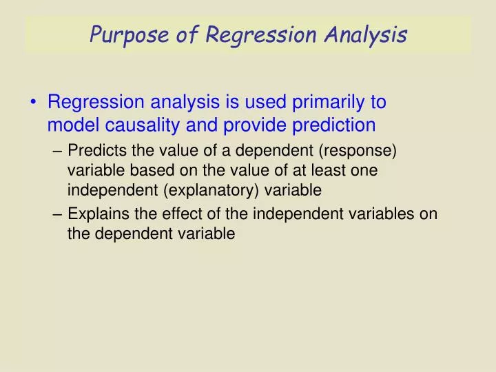
Purpose of Regression Analysis. Regression analysis is used primarily to model causality and provide prediction Predicts the value of a dependent (response) variable based on the value of at least one independent (explanatory) variable

E N D
Purpose of Regression Analysis • Regression analysis is used primarily to model causality and provide prediction • Predicts the value of a dependent (response) variable based on the value of at least one independent (explanatory) variable • Explains the effect of the independent variables on the dependent variable
Types of Regression Models Positive Linear Relationship Relationship NOT Linear Negative Linear Relationship No Relationship
Simple Linear Regression Model • Relationship between variables is described by a linear function • The change of one variable causes the change in the other variable • A dependency of one variable on the other
Population Linear Regression Population regression line is a straight line that describes the dependence of the average value (conditional mean) of one variable on the other Random Error Population SlopeCoefficient Population Y intercept Dependent (Response) Variable PopulationRegression Line (conditional mean) Independent (Explanatory) Variable
Population Linear Regression (continued) Y (Observed Value of Y) = = Random Error (Conditional Mean) X Observed Value of Y
Sample Linear Regression Sample regression line provides an estimate of the population regression line as well as a predicted value of Y SampleSlopeCoefficient Sample Y Intercept Residual Sample Regression Line (Fitted Regression Line, Predicted Value)
Sample Linear Regression (continued) • and are obtained by finding the values of and that minimizes the sum of the squared residuals • provides an estimate of • provides and estimate of
Sample Linear Regression (continued) Y X Observed Value
Interpretation of the Slope and the Intercept • is the average value of Y when the value of X is zero. • measures the change in the average value of Y as a result of a one-unit change in X.
Interpretation of the Slope and the Intercept (continued) • is the estimated average value of Y when the value of X is zero. • is the estimated change in the average value of Y as a result of a one-unit change in X.
Simple Linear Regression: Example You want to examine the linear dependency of the annual sales of produce stores on their size in square footage. Sample data for seven stores were obtained. Find the equation of the straight line that fits the data best. Annual Store Square Sales Feet ($1000) 1 1,726 3,681 2 1,542 3,395 3 2,816 6,653 4 5,555 9,543 5 1,292 3,318 6 2,208 5,563 7 1,313 3,760
Scatter Diagram: Example Excel Output
Equation for the Sample Regression Line: Example From Excel Printout:
Graph of the Sample Regression Line: Example Yi = 1636.415 +1.487Xi
Interpretation of Results: Example The slope of 1.487 means that for each increase of one unit in X, we predict the average of Y to increase by an estimated 1.487 units. The model estimates that for each increase of one square foot in the size of the store, the expected annual sales are predicted to increase by $1487.
How Good is the regression? • R2 • Confidence Intervals • Residual Plots • Analysis of Variance • Hypothesis (t) tests
Measure of Variation: The Sum of Squares SST =SSR + SSE Total Sample Variability Unexplained Variability = Explained Variability +
Measure of Variation: The Sum of Squares (continued) • SST = total sum of squares • Measures the variation of the Yi values around their mean Y • SSR = regression sum of squares • Explained variation attributable to the relationship between X and Y • SSE = error sum of squares • Variation attributable to factors other than the relationship between X and Y
Measure of Variation: The Sum of Squares (continued) Y SSE =(Yi-Yi )2 _ SST =(Yi-Y)2 _ SSR = (Yi -Y)2 _ Y X Xi
The Coefficient of Determination • Measures the proportion of variation in Y that is explained by the independent variable X in the regression model
Coefficients of Determination (r 2) and Correlation (r) r2 = 1, Y r = +1 Y r2 = 1, r = -1 ^ Y = b + b X i 0 1 i ^ Y = b + b X i 0 1 i X X r2 = .8, r2 = 0, r = +0.9 r = 0 Y Y ^ ^ Y = b + b X Y = b + b X i 0 1 i i 0 1 i X X
Linear Regression Assumptions • Linearity • Normality • Y values are normally distributed for each X • Probability distribution of error is normal 2. Homoscedasticity (Constant Variance) 3. Independence of Errors
Residual Analysis • Purposes • Examine linearity • Evaluate violations of assumptions • Graphical Analysis of Residuals • Plot residuals vs. Xi , Yi and time
Residual Analysis for Linearity Y Y X X e e X X Not Linear Linear
Residual Analysis for Homoscedasticity Y Y X X SR SR X X Homoscedasticity Heteroscedasticity
Variation of Errors around the Regression Line • Y values are normally distributed around the regression line. • For each X value, the “spread” or variance around the regression line is the same. f(e) Y X2 X1 X Sample Regression Line
Residual Analysis:Excel Output for Produce Stores Example Excel Output
Residual Analysis for Independence Graphical Approach Not Independent Independent e e Time Time Cyclical Pattern No Particular Pattern Residual is plotted against time to detect any autocorrelation
Inference about the Slope: t Test • t test for a population slope • Is there a linear dependency of Y on X ? • Null and alternative hypotheses • H0: 1 = 0 (no linear dependency) • H1: 1 0 (linear dependency) • Test statistic
Example: Produce Store Data for Seven Stores: Estimated Regression Equation: Annual Store Square Sales Feet ($000) 1 1,726 3,681 2 1,542 3,395 3 2,816 6,653 4 5,555 9,543 5 1,292 3,318 6 2,208 5,563 7 1,313 3,760 Yi = 1636.415 +1.487Xi The slope of this model is 1.487. Is square footage of the store affecting its annual sales?
H0: 1 = 0 H1: 1 0 .05 df7 - 2 = 5 Critical Value(s): Inferences about the Slope: t Test Example Test Statistic: Decision: Conclusion: From Excel Printout Reject H0 Reject Reject .025 .025 There is evidence that square footage affects annual sales. t -2.5706 0 2.5706
The Multiple Regression Model Relationship between 1 dependent & 2 or more independent variables is a linear function Population Y-intercept Population slopes Random Error Residual Dependent (Response) variable for sample Independent (Explanatory) variables for sample model
Population Multiple Regression Model Bivariate model
Sample Multiple Regression Model Bivariate model Sample Regression Plane
Simple and Multiple Regression Compared • Coefficients in a simple regression pick up the impact of that variable plus the impacts of other variables that are correlated with it and the dependent variable. • Coefficients in a multiple regression net out the impacts of other variables in the equation.
Simple and Multiple Regression Compared:Example • Two simple regressions: • Multiple regression:
Multiple Linear Regression Equation Too complicated by hand! Ouch!
Interpretation of Estimated Coefficients • Slope (bi) • Estimated that the average value of Y changes by bi for each 1 unit increase in Xi holding all other variables constant (ceteris paribus) • Example: if b1 = -2, then fuel oil usage (Y) is expected to decrease by an estimated 2 gallons for each 1 degree increase in temperature (X1) given the inches of insulation (X2) • Y-intercept (b0) • The estimated average value of Y when all Xi = 0
Multiple Regression Model: Example (0F) Develop a model for estimating heating oil used for a single family home in the month of January based on average temperature and amount of insulation in inches.
Sample Multiple Regression Equation: Example Excel Output For each degree increase in temperature, the estimated average amount of heating oil used is decreased by 5.437 gallons, holding insulation constant. For each increase in one inch of insulation, the estimated average use of heating oil is decreased by 20.012 gallons, holding temperature constant.
Confidence Interval Estimate for the Slope Provide the 95% confidence interval for the population slope 1(the effect of temperature on oil consumption). -6.169 1 -4.704 The estimated average consumption of oil is reduced by between 4.7 gallons to 6.17 gallons per each increase of 10 F.
Coefficient of Multiple Determination • Proportion of total variation in Y explained by all X variables taken together • Never decreases when a new X variable is added to model • Disadvantage when comparing models
Adjusted Coefficient of Multiple Determination • Proportion of variation in Y explained by all X variables adjusted for the number of X variables used • Penalize excessive use of independent variables • Smaller than • Useful in comparing among models
Coefficient of Multiple Determination Excel Output • Adjusted r2 • reflects the number of explanatory variables and sample size • is smaller than r2
Interpretation of Coefficient of Multiple Determination • 96.56% of the total variation in heating oil can be explained by different temperature and amount of insulation • 95.99% of the total fluctuation in heating oil can be explained by different temperature and amount of insulation after adjusting for the number of explanatory variables and sample size
Using The Model to Make Predictions Predict the amount of heating oil used for a home if the average temperature is 300 and the insulation is six inches. The predicted heating oil used is 278.97 gallons
Testing for Overall Significance • Shows if there is a linear relationship between all of the X variables together and Y • Use F test statistic • Hypotheses: • H0: 1 = 2 = … = k = 0 (no linear relationship) • H1: at least one i 0 ( at least one independent variable affects Y ) • The null hypothesis is a very strong statement • Almost always reject the null hypothesis
Test for Significance:Individual Variables • Shows if there is a linear relationship between the variable Xi and Y • Use t test statistic • Hypotheses: • H0: i= 0 (no linear relationship) • H1: i 0 (linear relationship between Xi and Y)
Residual Plots • Residuals vs. • May need to transform variable • Residuals vs. • May need to transform variable • Residuals vs. time • May have autocorrelation