Download
1 / 34
400 likes | 948 Vues
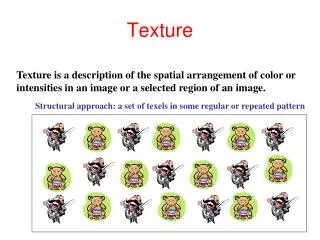
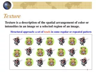
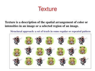
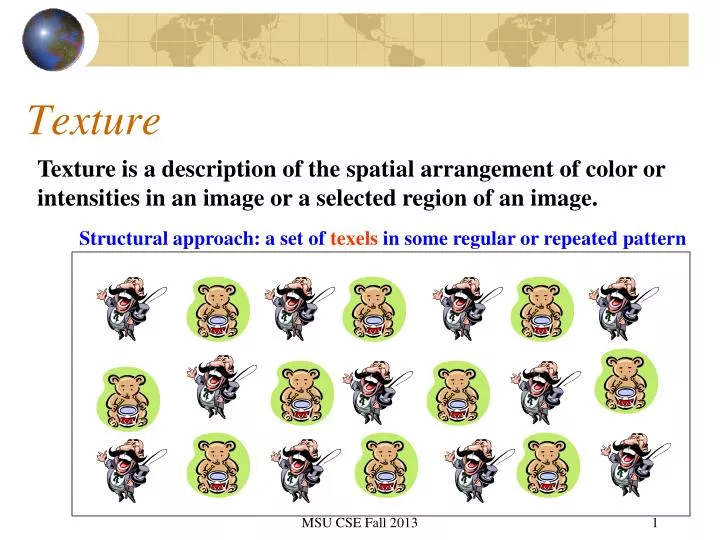
Texture. Texture is a description of the spatial arrangement of color or intensities in an image or a selected region of an image. Structural approach: a set of texels in some regular or repeated pattern. Why Texture Analysis?. Aspects of texture.

E N D
Texture Texture is a description of the spatial arrangement of color or intensities in an image or a selected region of an image. Structural approach: a set of texels in some regular or repeated pattern MSU CSE Fall 2013
Why Texture Analysis? MSU CSE Fall 2013
Aspects of texture • Size or granularity (sand versus pebbles versus boulders) • Directionality (stripes versus sand) • Random or regular (sawdust versus woodgrain; stucko versus bricks) • Concept of texture elements (texel) and spatial arrangement of texels MSU CSE Fall 2013
Problem with Structural Approach How do you decide what is a texel? Ideas? MSU CSE Fall 2013
Natural Textures grass leaves What/Where are the texels? MSU CSE Fall 2013
The Case for Statistical Texture • Segmenting out texels is difficult or impossible in real images. • Numeric quantities or statistics that describe a texture can be • computed from the gray tones (or colors) alone. • This approach is less intuitive, but is computationally efficient. • It can be used for both classification and segmentation. MSU CSE Fall 2013
Some Simple Statistical Texture Measures 1. Edge Density and Direction • Use an edge detector as the first step in texture analysis. • The number of edge pixels in a fixed-size region tells us • how busy that region is. • The directions of the edges also help characterize the texture MSU CSE Fall 2013
Two Edge-based Texture Measures 1. edgeness per unit area 2. edge magnitude and direction histograms Fedgeness = |{ p | gradient_magnitude(p) threshold}| / N where N is the size of the unit area Fmagdir = ( Hmagnitude, Hdirection ) where these are the normalized histograms of gradient magnitudes and gradient directions, respectively. How would you compare two histograms? MSU CSE Fall 2013
Examples Fe = 25/25 Fe = 6/25 Hm = (6,19)/25 Hm = (0,6)/25 Hd = (12,13,0)/25 Hd = (0,0,6)/25 MSU CSE Fall 2013
Original Image Frei-Chen Thresholded Edge Image Edge Image MSU CSE Fall 2013
Local Binary Partition Measure • For each pixel p, create an 8-bit number b1 b2 b3 b4 b5 b6 b7 b8, • where bi = 0 if neighbor i has value less than or equal to p’s • value and 1 otherwise. • Represent the texture in the image (or a region) by the • histogram of these numbers. 1 2 3 100 101 103 40 50 80 50 60 90 4 5 1 1 1 1 1 1 0 0 8 7 6 MSU CSE Fall 2013
Fids (Flexible Image Database System) is retrieving images similar to the query image using LBP texture as the texture measure and comparing their LBP histograms MSU CSE Fall 2013
Low-level measures don’t always find semantically similar images. MSU CSE Fall 2013
Co-occurrence Matrix Features A co-occurrence matrix is a 2D array C in which • Both the rows and columns represent a set of possible • image values • C (i,j) indicates how many times value i co-occurs with • value j in a particular spatial relationship d. • The spatial relationship is specified by a vector d = (dr,dc). d MSU CSE Fall 2013
1 0 1 2 1 1 0 0 1 1 0 0 0 0 2 2 0 0 2 2 0 0 2 2 0 0 2 2 i j 0 1 2 1 0 3 2 0 2 0 0 1 3 C d co-occurrence matrix d = (3,1) gray-tone image From C we can compute N , the normalized co-occurrence matrix, where each value is divided by the sum of all the values. d d MSU CSE Fall 2013
Co-occurrence Features What do these measure? sums. Energy measures uniformity of the normalized matrix. MSU CSE Fall 2013
But how do you choose d? • This is actually a critical question with all the • statistical texture methods. • Are the “texels” tiny, medium, large, all three …? • Not really a solved problem. Zucker and Terzopoulos suggested using a statistical test to select the value(s) of d that have the most structure for a given class of images. See transparencies. 2 MSU CSE Fall 2013
Laws’ Texture Energy Features • Signal-processing-based algorithms use texture filters • applied to the image to create filtered images from which • texture features are computed. • The Laws Algorithm • Filter the input image using texture filters. • Compute texture energy by summing the absolute • value of filtering results in local neighborhoods • around each pixel. • Combine features to achieve rotational invariance. MSU CSE Fall 2013
Law’s texture masks (1) MSU CSE Fall 2013
Law’s texture masks (2) Creation of 2D Masks E5 L5 E5L5 MSU CSE Fall 2013
9D feature vector for pixel • Subtract mean neighborhood intensity from pixel • Dot product 16 5x5 masks with neighborhood • 9 features defined as follows: MSU CSE Fall 2013
Features from sample images MSU CSE Fall 2013
water tiger fence flag grass Is there a neighborhood size problem with Laws? small flowers big flowers MSU CSE Fall 2013
Autocorrelation function • Autocorrelation function can detect repetitive patterns of texels • Also defines fineness/coarseness of the texture • Compare the dot product (energy) of non shifted image with a shifted image MSU CSE Fall 2013
Interpreting autocorrelation • Coarse texture function drops off slowly • Fine texture function drops off rapidly • Can drop differently for r and c • Regular textures function will have peaks and valleys; peaks can repeat far away from [0, 0] • Random textures only peak at [0, 0]; breadth of peak gives the size of the texture MSU CSE Fall 2013
Fourier power spectrum • High frequency power fine texture • Concentrated power regularity • Directionality directional texture MSU CSE Fall 2013
Fourier example MSU CSE Fall 2013
Notes on Texture by FFT The power spectrum computed from the Fourier Transform reveals which waves represent the image energy. MSU CSE Fall 2013
Stripes of the zebra create high energy waves generally along the u-axis; grass pattern is fairly random causing scattered low frequency energy y x v u MSU CSE Fall 2013
More stripes Power spectrum x 64 MSU CSE Fall 2013
Spectrum shows broad energy along u axis and less along the v-axis: the roads give more structure vertically and so does the regularity of the houses MSU CSE Fall 2013
Spartan stadium: the pattern of the seats is evident in the power spectrum – lots of energy in (u,v) along the direction of the seats. MSU CSE Fall 2013
Getting features from the spectrum • FT can be applied to square image regions to extract texture features • set conditions on u-v transform image to compute features: f1 = sum of all pixels where R1 < || (u,v)|| < R2 (bandpass) • f2 = sum of pixels (u,v) where u1 < u <u2 • f3 = sum of pixels where ||(u,v)-(u0,v0)|| < R MSU CSE Fall 2013
Filtering or feature extraction using special regions of u-v F4 is all energy in directional wedge F1 is all energy in small circle F2 is all energy near origin (low pass) F3 is all energy outside circle (high pass) MSU CSE Fall 2013